Visualizing 3D Genome Organization with gghic

Introduction

gghic is an R package for creating publication-ready visualizations of 3D genome organization data. It seamlessly integrates Hi-C contact maps, topologically associating domains (TADs), chromatin loops, gene annotations, and genomic tracks into unified, customizable plots.

Why gghic?

Easy to use: Simple, intuitive syntax with sensible defaults for quick plotting
Flexible: Choose between high-level gghic() wrapper or low-level geom_* layers for fine control
Memory efficient: Smart focus mechanism loads only the genomic regions you need
Publication-ready: High-quality figures with minimal code
Extensible: Built on ggplot2 ecosystem—use standard ggplot2 functions for customization

Key Features

ChromatinContacts S4 class: Robust object-oriented framework for managing Hi-C/-like data
Flexible focusing: Efficiently subset genomic regions before or after loading data
Feature integration: Seamlessly combine TADs, loops, genes, and signal tracks
Multiple visualization modes: Single chromosome, multi-chromosome, inter-chromosomal, and multi-way contacts
Hypergraph analysis: Specialized tools for visualizing Pore-C/-like multi-way chromatin interactions

Resources:

arXiv preprint

GitHub repository

Depth by resolution vignette for Hi-C/-like data quality assessment

Hypergraph vignette for Pore-C/-like multi-way contact analysis

Typical Workflow

Load data: Create ChromatinContacts object from Cooler files
Focus: Specify genomic regions of interest (optional but recommended)
Import: Load interaction data into memory
Add features: Attach TADs, loops, genes, and tracks (optional)
Visualize: Use gghic() wrapper or custom ggplot2 layers
Customize: Refine with standard ggplot2 functions and themes

Getting Started

Load Required Packages

load_pkg <- function(pkgs) {
  for (pkg in pkgs) suppressMessages(require(pkg, character.only = TRUE))
}

load_pkg(
  c("ggplot2", "dplyr", "GenomicRanges", "InteractionSet", "gghic")
)

Download Example data

The example data files are hosted on the gghic-data repository. This function downloads files to a local cache:

download_example_files <- function(cache_dir, check_exists = TRUE) {
  if (!dir.exists(cache_dir)) dir.create(cache_dir, recursive = TRUE)

  files <- list(
    "chr4_11-100kb.cool" = "cooler/chr4_11-100kb.cool",
    "chr4_11-5kb.cool" = "cooler/chr4_11-5kb.cool",
    "track1.bigWig" = "bigwig/track1.bigWig",
    "track2.bigWig" = "bigwig/track2.bigWig",
    "gencode-chr4_11.gtf.gz" = "gtf/gencode-chr4_11.gtf.gz",
    "TADs_500kb-chr4_11.tsv" = "tad/TADs_500kb-chr4_11.tsv",
    "loops-chr4_11.txt" = "loop/loops-chr4_11.txt",
    "gis_hic.rds" = "multiway/gis_hic.rds",
    "concatemers.rds" = "multiway/concatemers.rds"
  )

  url_base <- "https://raw.githubusercontent.com/mhjiang97/gghic-data/master/"

  for (file_name in names(files)) {
    file_path <- file.path(cache_dir, file_name)
    if (check_exists && file.exists(file_path)) next
    message("Downloading ", file_name, "...")
    download.file(
      paste0(url_base, files[[file_name]]), file_path,
      method = "curl", quiet = TRUE
    )
  }
}

# Define a cache directory and download the files
dir_cache <- file.path("..", "data")
download_example_files(dir_cache)

# Set up paths to the downloaded files
path_cf_100 <- file.path(dir_cache, "chr4_11-100kb.cool")
path_cf_5 <- file.path(dir_cache, "chr4_11-5kb.cool")
path_gtf <- file.path(dir_cache, "gencode-chr4_11.gtf.gz")
paths_track <- file.path(dir_cache, paste0("track", 1:2, ".bigWig"))
path_tad <- file.path(dir_cache, "TADs_500kb-chr4_11.tsv")
path_loop <- file.path(dir_cache, "loops-chr4_11.txt")
path_gis_hic <- file.path(dir_cache, "gis_hic.rds")
path_concatemers <- file.path(dir_cache, "concatemers.rds")

Working with ChromatinContacts Objects

Understanding ChromatinContacts

The ChromatinContacts object is the central data structure in gghic. It acts as a lightweight pointer to your Hi-C data (Cooler files), storing resolution and sequence information without loading the massive interaction matrix into memory immediately.

A key feature is the focus argument. This allows you to specify chromosomes or regions of interest before importing the data.

Why use focus?

Speed: Only reads relevant parts of the Hi-C matrix.
Memory Efficiency: Prevents loading genome-wide matrices when you only need a specific locus.

Creating ChromatinContacts Objects

No Focus (Genome-Wide)

Without a focus, the object references the entire genome:

cc_100_all <- ChromatinContacts(cooler_path = path_cf_100)
cc_100_all
#> ChromatinContacts object
#> --------------------------------------------------
#> File: chr4_11-100kb.cool
#> Sequences: 2 (chr11, chr4)
#> Focus: genome-wide
#> Interactions: not loaded (use import() to load)
#> --------------------------------------------------

Focusing on Specific Regions

The focus argument accepts flexible region specifications. This is the recommended approach for working with large Hi-C datasets.

Single Region or Chromosome

# Focus on entire chromosome (includes all intra-chromosomal interactions)
cc_chr11 <- ChromatinContacts(cooler_path = path_cf_100, focus = "chr11")
cc_chr11
#> ChromatinContacts object
#> --------------------------------------------------
#> File: chr4_11-100kb.cool
#> Sequences: 2 (chr11, chr4)
#> Focus: 1 region
#>   [1] chr11:1:135,006,516 <-> chr11:1:135,006,516
#> Interactions: not loaded (use import() to load)
#> --------------------------------------------------

# Focus on specific 10 Mb region
cc_chr11_region <- ChromatinContacts(
  cooler_path = path_cf_100, focus = "chr11:60000000-70000000"
)
cc_chr11_region
#> ChromatinContacts object
#> --------------------------------------------------
#> File: chr4_11-100kb.cool
#> Sequences: 2 (chr11, chr4)
#> Focus: 1 region
#>   [1] chr11:60,000,000:70,000,000 <-> chr11:60,000,000:70,000,000
#> Interactions: not loaded (use import() to load)
#> --------------------------------------------------

Multiple Regions with Operators

Use | (OR) for multiple regions and & (AND) for inter-regional interactions:

# Multiple chromosomes
# Returns: chr4-chr4, chr11-chr11, AND chr4-chr11 interactions
cc_multi <- ChromatinContacts(
  cooler_path = path_cf_100, focus = "chr4 | chr11"
)
cc_multi
#> ChromatinContacts object
#> --------------------------------------------------
#> File: chr4_11-100kb.cool
#> Sequences: 2 (chr11, chr4)
#> Focus: 3 regions
#>   [1] chr11:1:135,006,516 <-> chr11:1:135,006,516
#>   [2] chr11:1:135,006,516 <-> chr4:1:191,154,276
#>   [3] chr4:1:191,154,276 <-> chr4:1:191,154,276
#> Interactions: not loaded (use import() to load)
#> --------------------------------------------------

# Inter-chromosomal interactions ONLY (no intra-chromosomal)
cc_inter <- ChromatinContacts(
  cooler_path = path_cf_100,
  focus = "chr4:10000000-15000000 & chr11:60000000-65000000"
)
cc_inter
#> ChromatinContacts object
#> --------------------------------------------------
#> File: chr4_11-100kb.cool
#> Sequences: 2 (chr11, chr4)
#> Focus: 1 region
#>   [1] chr11:60,000,000:65,000,000 <-> chr4:10,000,000:15,000,000
#> Interactions: not loaded (use import() to load)
#> --------------------------------------------------

Complex Focus Patterns

Combine operators for sophisticated queries:

# Example 1: Multiple intra-chromosomal + one trans-chromosomal
# Returns: chr1-chr1, chr2-chr2, chr3-chr3, chr1-chr2, chr1-chr3, chr2-chr3, AND chr4-chr5
focus_complex <- c("chr1 | chr2 | chr3", "chr4 & chr5")

# Example 2: Specific regions with trans interactions
focus <- c(
  "chr1:1000000-5000000 | chr2:3000000-8000000",
  "chr3:10000000-15000000 & chr4:20000000-25000000"
)

# Example 3: Multiple trans-chromosomal pairs
focus <- c("chr1 & chr2", "chr3 & chr4", "chr5 & chr6")

💡 Practical Tips:

Use focus when working with genome-wide data files (saves time and memory)
For exploratory analysis, start with whole chromosome, then zoom to regions
Use & operator when specifically studying trans-chromosomal interactions
Combine focusing with subsetting (next section) for iterative analysis

Using GInteractions Objects

For programmatic region definition (useful in pipelines):

# Create a GInteractions object to specify the focus
focus_gi <- suppressWarnings(InteractionSet::GInteractions(
  GenomicRanges::GRanges("chr4:10000000-12000000"),
  GenomicRanges::GRanges("chr11:61000000-63000000")
))

cc_gis_focus <- ChromatinContacts(
  cooler_path = path_cf_100,
  focus = focus_gi
)
cc_gis_focus
#> ChromatinContacts object
#> --------------------------------------------------
#> File: chr4_11-100kb.cool
#> Sequences: 2 (chr11, chr4)
#> Focus: 1 region
#>   [1] chr4:10,000,000:12,000,000 <-> chr11:61,000,000:63,000,000
#> Interactions: not loaded (use import() to load)
#> --------------------------------------------------

Import Interaction Data

After creating the object, use import() to load the actual data:

cc_100 <- import(cc_100_all)
cc_100
#> ChromatinContacts object
#> --------------------------------------------------
#> File: chr4_11-100kb.cool
#> Resolution: 100,000 bp
#> Sequences: 2 (chr11, chr4)
#> Focus: genome-wide
#> Interactions: 1,150,956 interactions
#>   Metadata columns: bin_id1, bin_id2, count, balanced
#> --------------------------------------------------

# Chain operations with pipe operator
cc_5 <- ChromatinContacts(cooler_path = path_cf_5) |>
  import()
cc_5
#> ChromatinContacts object
#> --------------------------------------------------
#> File: chr4_11-5kb.cool
#> Resolution: 5,000 bp
#> Sequences: 2 (chr11, chr4)
#> Focus: genome-wide
#> Interactions: 4,825,031 interactions
#>   Metadata columns: bin_id1, bin_id2, count, balanced
#> --------------------------------------------------

Adding Genomic Features

Attach genomic features (TADs, loops, tracks) to your ChromatinContacts object for integrated visualization.

Key Benefits:

Automatic synchronization: Features are automatically subsetted when you zoom or change regions
Consistent context: All features stay aligned with the contact map
Simplified plotting: Pass a single object to gghic() instead of managing multiple data sources

# Load TADs, loops, and tracks from files
tads <- rtracklayer::import(path_tad, format = "bed")
loops <- path_loop |>
  rtracklayer::import(format = "bedpe") |>
  makeGInteractionsFromGRangesPairs()
tracks <- paths_track |>
  purrr::map(rtracklayer::import) |>
  setNames(paste0("track", seq_along(paths_track))) |>
  GenomicRanges::GRangesList()

# Add features to the ChromatinContacts object
features(cc_100, "TADs") <- tads
features(cc_100, "loops") <- loops
features(cc_100, "tracks") <- tracks

cc_100
#> ChromatinContacts object
#> --------------------------------------------------
#> File: chr4_11-100kb.cool
#> Resolution: 100,000 bp
#> Sequences: 2 (chr11, chr4)
#> Focus: genome-wide
#> Interactions: 1,150,956 interactions
#>   Metadata columns: bin_id1, bin_id2, count, balanced
#> Features:
#>   TADs: 245 regions
#>   Loops: 255 regions
#>   Tracks: 2 regions
#>   Tracks: 2 tracks
#>     [1] track1: 2,403,441 ranges
#>     [2] track2: 1,884,707 ranges
#> --------------------------------------------------

features(cc_5, "TADs") <- tads
features(cc_5, "loops") <- loops
features(cc_5, "tracks") <- tracks

Manipulating ChromatinContacts Objects

ChromatinContacts objects support flexible subsetting after data import. This is useful for:

Iterative exploration: Start broad, then zoom to interesting regions
Comparative analysis: Extract same region from multiple samples
Quality filtering: Remove low-quality or extreme-valued interactions

Automatic updates: Subsetting filters interactions AND updates:

Associated features (TADs, loops, tracks)
The focus slot (tracks current genomic context)
Sequence information (seqinfo)

Subsetting by Genomic Regions (character)

The most intuitive way to subset is by providing a character string representing a genomic region:

# Subset to keep only interactions on chromosome 11
cc_chr11 <- cc_100["chr11"]
cc_chr11
#> ChromatinContacts object
#> --------------------------------------------------
#> File: chr4_11-100kb.cool
#> Resolution: 100,000 bp
#> Sequences: 2 (chr11, chr4)
#> Focus: 1 region
#>   [1] chr11:1:135,006,516 <-> chr11:1:135,006,516
#> Interactions: 328,865 interactions
#>   Metadata columns: bin_id1, bin_id2, count, balanced
#> Features:
#>   TADs: 107 regions
#>   Loops: 134 regions
#>   Tracks: 2 regions
#>   Tracks: 2 tracks
#>     [1] track1: 1,332,687 ranges
#>     [2] track2: 985,360 ranges
#> --------------------------------------------------

# Subset to a specific 20 Mb region on chromosome 4
cc_chr4_sub <- cc_100["chr4:20000000-40000000"]
cc_chr4_sub
#> ChromatinContacts object
#> --------------------------------------------------
#> File: chr4_11-100kb.cool
#> Resolution: 100,000 bp
#> Sequences: 2 (chr11, chr4)
#> Focus: 1 region
#>   [1] chr4:1:191,154,276 <-> chr4:1:191,154,276
#> Interactions: 17,012 interactions
#>   Metadata columns: bin_id1, bin_id2, count, balanced
#> Features:
#>   TADs: 17 regions
#>   Loops: 7 regions
#>   Tracks: 2 regions
#>   Tracks: 2 tracks
#>     [1] track1: 111,157 ranges
#>     [2] track2: 89,885 ranges
#> --------------------------------------------------

Subsetting with GRanges

You can use a GRanges object to subset interactions where at least one anchor overlaps the given ranges:

# Define a region of interest
roi <- GenomicRanges::GRanges("chr11:60000000-70000000")

# Subset the ChromatinContacts object
cc_gr_sub <- cc_100[roi]
cc_gr_sub
#> ChromatinContacts object
#> --------------------------------------------------
#> File: chr4_11-100kb.cool
#> Resolution: 100,000 bp
#> Sequences: 2 (chr11, chr4)
#> Focus: 1 region
#>   [1] chr11:1:135,006,516 <-> chr11:1:135,006,516
#> Interactions: 4,215 interactions
#>   Metadata columns: bin_id1, bin_id2, count, balanced
#> Features:
#>   TADs: 8 regions
#>   Loops: 58 regions
#>   Tracks: 2 regions
#>   Tracks: 2 tracks
#>     [1] track1: 299,741 ranges
#>     [2] track2: 165,088 ranges
#> --------------------------------------------------

Subsetting with GInteractions

To select a specific set of interactions, you can subset using a GInteractions object. This will keep only the interactions from the ChromatinContacts object that overlap with the query GInteractions:

# Define a specific inter-chromosomal interaction to query
query_gi <- InteractionSet::GInteractions(
  GenomicRanges::GRanges("chr11:60000000-65000000"),
  GenomicRanges::GRanges("chr4:10000000-15000000")
)

# Subset the object
cc_gi_sub <- cc_100[query_gi]

cc_gi_sub
#> ChromatinContacts object
#> --------------------------------------------------
#> File: chr4_11-100kb.cool
#> Resolution: 100,000 bp
#> Sequences: 2 (chr11, chr4)
#> Focus: 1 region
#>   [1] chr11:1:135,006,516 <-> chr4:1:191,154,276
#> Interactions: 89 interactions
#>   Metadata columns: bin_id1, bin_id2, count, balanced
#> Features:
#>   TADs: 10 regions
#>   Tracks: 2 regions
#>   Tracks: 2 tracks
#>     [1] track1: 108,442 ranges
#>     [2] track2: 70,400 ranges
#> --------------------------------------------------

Subsetting by Index or Logical Vector

You can also use numeric indices or logical vectors for subsetting, similar to how you would subset a data.frame or a vector:

# Subset by numeric index (e.g., first 1000 interactions)
cc_numeric_sub <- cc_100[1:100]

cc_numeric_sub
#> ChromatinContacts object
#> --------------------------------------------------
#> File: chr4_11-100kb.cool
#> Resolution: 100,000 bp
#> Sequences: 2 (chr11, chr4)
#> Focus: 2 regions
#>   [1] chr11:1:135,006,516 <-> chr11:1:135,006,516
#>   [2] chr11:1:135,006,516 <-> chr4:1:191,154,276
#> Interactions: 100 interactions
#>   Metadata columns: bin_id1, bin_id2, count, balanced
#> Features:
#>   TADs: 55 regions
#>   Tracks: 2 regions
#>   Tracks: 2 tracks
#>     [1] track1: 123,248 ranges
#>     [2] track2: 79,981 ranges
#> --------------------------------------------------

# Subset using a logical vector (e.g., interactions with a score > -0.1)
df <- scaleData(cc_100, "balanced", log10)

# Then subset based on the score
logical_vec <- (df$score > -0.1) & !is.na(df$score)
cc_logical_sub <- cc_100[logical_vec]

cc_logical_sub
#> ChromatinContacts object
#> --------------------------------------------------
#> File: chr4_11-100kb.cool
#> Resolution: 100,000 bp
#> Sequences: 2 (chr11, chr4)
#> Focus: 2 regions
#>   [1] chr11:1:135,006,516 <-> chr11:1:135,006,516
#>   [2] chr4:1:191,154,276 <-> chr4:1:191,154,276
#> Interactions: 25 interactions
#>   Metadata columns: bin_id1, bin_id2, count, balanced
#> Features:
#>   TADs: 13 regions
#>   Loops: 2 regions
#>   Tracks: 2 regions
#>   Tracks: 2 tracks
#>     [1] track1: 53,256 ranges
#>     [2] track2: 30,979 ranges
#> --------------------------------------------------

Creating Visualizations

gghic provides two complementary approaches for plotting:

Visualization Approaches

1. High-Level Wrapper: `gghic()`

Best for: Quick plots, standard layouts, exploratory analysis

Single function call with sensible defaults
Automatically handles data scaling and transformation
Optional arguments for ideograms, genes, TADs, loops, and tracks
Returns a ggplot2 object for further customization

2. Low-Level Layers: `geom_*()`

Best for: Custom layouts, complex multi-panel figures, precise control

Build plots layer-by-layer like standard ggplot2
Full control over aesthetics, scales, and themes
Mix with other ggplot2 geoms and extensions
Ideal for publication figures with specific requirements

Basic Hi-C Heatmap

Using `geom_hic()` Layer

geom_hic() creates the triangle heatmap visualization. It works with standard data frames/tibbles:

Required aesthetics: - seqnames1, start1, end1: First genomic anchor - seqnames2, start2, end2: Second genomic anchor - fill: Interaction strength (typically log-transformed)

df_100 <- cc_100 |>
  scaleData("balanced", log10)

p <- df_100 |>
  dplyr::filter(seqnames1 == "chr11", seqnames2 == "chr11") |>
  ggplot2::ggplot(
    ggplot2::aes(
      seqnames1 = seqnames1, start1 = start1, end1 = end1,
      seqnames2 = seqnames2, start2 = start2, end2 = end2, fill = score
    )
  ) +
  geom_hic()

p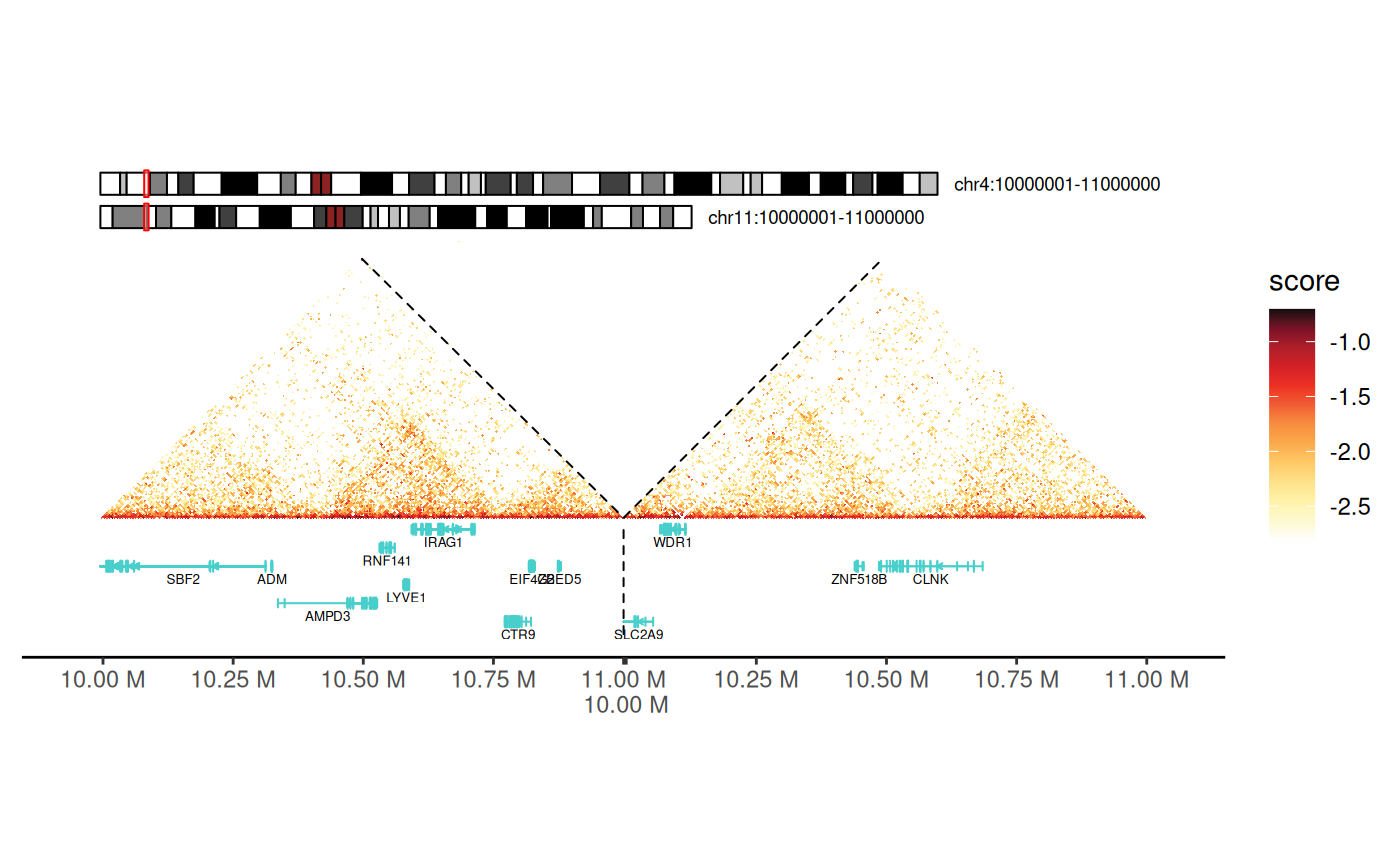

Hi-C visualization

theme_hic() provides a clean, publication-ready appearance:

Removes axis labels and tick marks
Eliminates grid lines
Focuses attention on the contact map
Suitable for most Hi-C visualizations

p + theme_hic()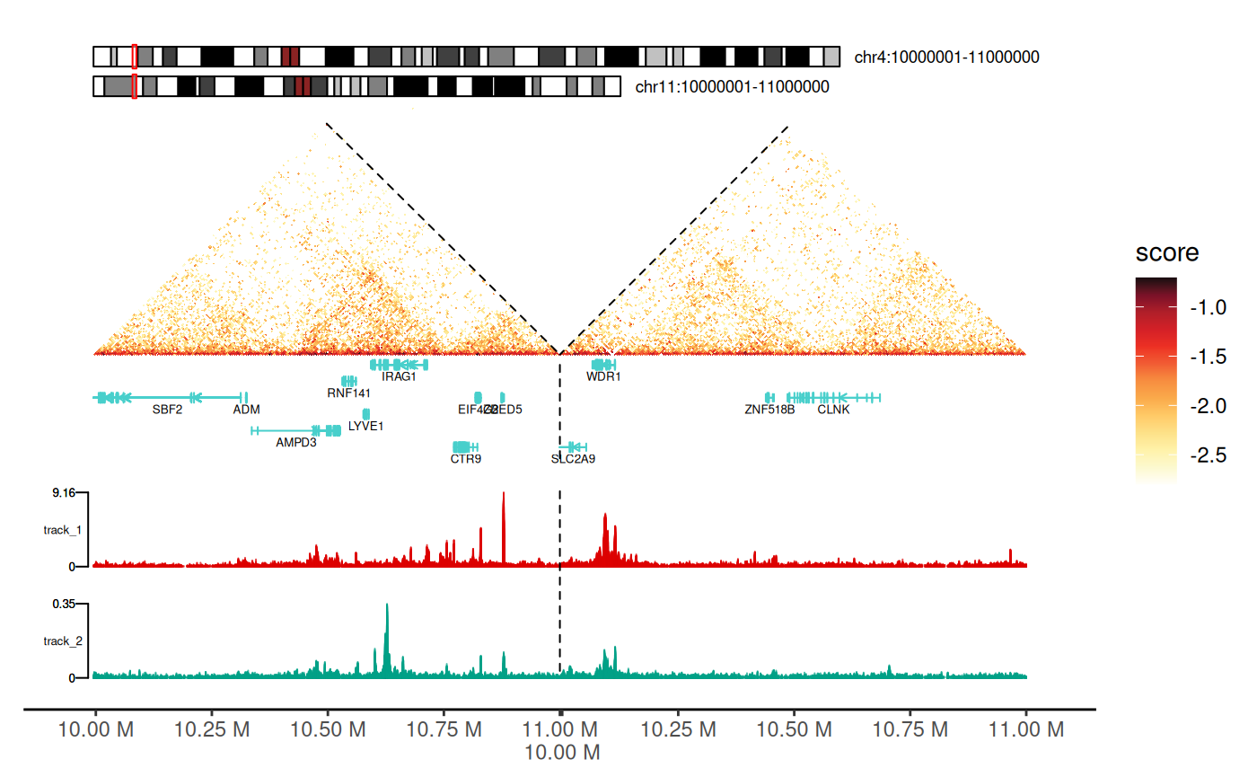

Hi-C visualization

Using `gghic()` Wrapper

The wrapper handles scaling and plotting automatically:

cc_100["chr11"] |>
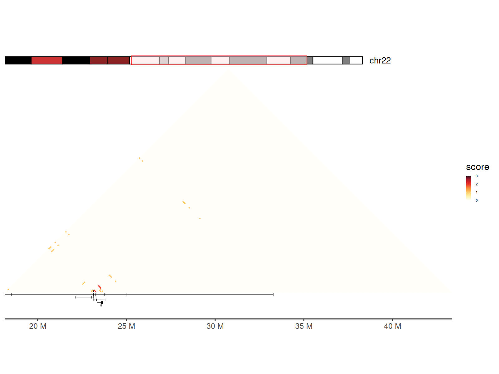
  gghic()

Adding Chromosome Ideograms

Chromosome ideograms provide genomic context by showing: - The entire chromosome with cytogenetic bands - Current viewing region highlighted - Chromosome name and position

Using `geom_ideogram()` Layer

Key parameters: - genome: Reference genome (“hg19”, “hg38”, “mm10”, “mm39”) - highlight: Whether to show the current region as a colored bar - length_ratio: Ideogram height relative to plot (0-1) - fontsize: Text size for chromosome labels

cc_100["chr4:10000000-15000000"] |>
  gghic() +
  geom_ideogram(
    genome = "hg19", highlight = TRUE, length_ratio = 0.7, fontsize = 8
  )

Hi-C visualization

Using the `ideogram` Argument in `gghic()`

cc_100["chr4:10000000-15000000"] |>
  gghic(
    ideogram = TRUE, genome = "hg19", highlight = TRUE,
    length_ratio = 0.7, ideogram_fontsize = 8
  )

Adding Gene Annotations

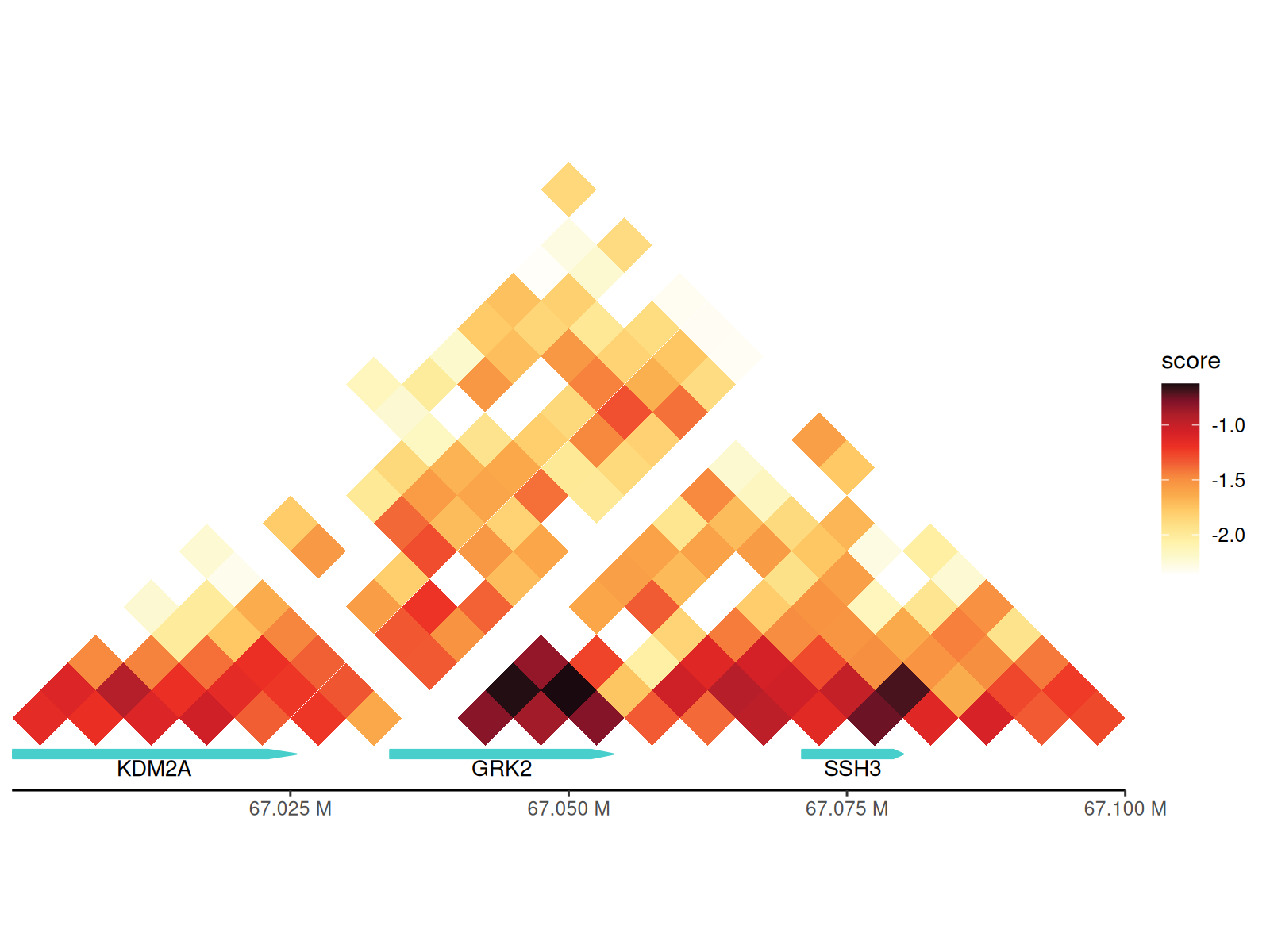
Visualize gene structures to correlate chromatin interactions with genomic features.

Annotation features: - Exon blocks (thick rectangles) - Introns (connecting lines) - Gene directionality (arrows for style = "arrow") - Multiple gene tracks for overlapping genes - Automatic collision detection and layout

Using `geom_annotation()` Layer

# Prepare data at 5kb resolution
df_5 <- cc_5 |>
  scaleData("balanced", log10)

# Create a base plot for a small region
p <- df_5 |>
  dplyr::filter(
    seqnames1 == "chr11", seqnames2 == "chr11",
    start1 > 67000000, start1 < 67100000,
    start2 > 67000000, start2 < 67100000
  ) |>
  ggplot(aes(
    seqnames1 = seqnames1, start1 = start1, end1 = end1,
    seqnames2 = seqnames2, start2 = start2, end2 = end2, fill = score
  )) +
  geom_hic() +
  theme_hic()

# Add the annotation layer
p + geom_annotation(gtf_path = path_gtf, style = "basic", maxgap = 100000)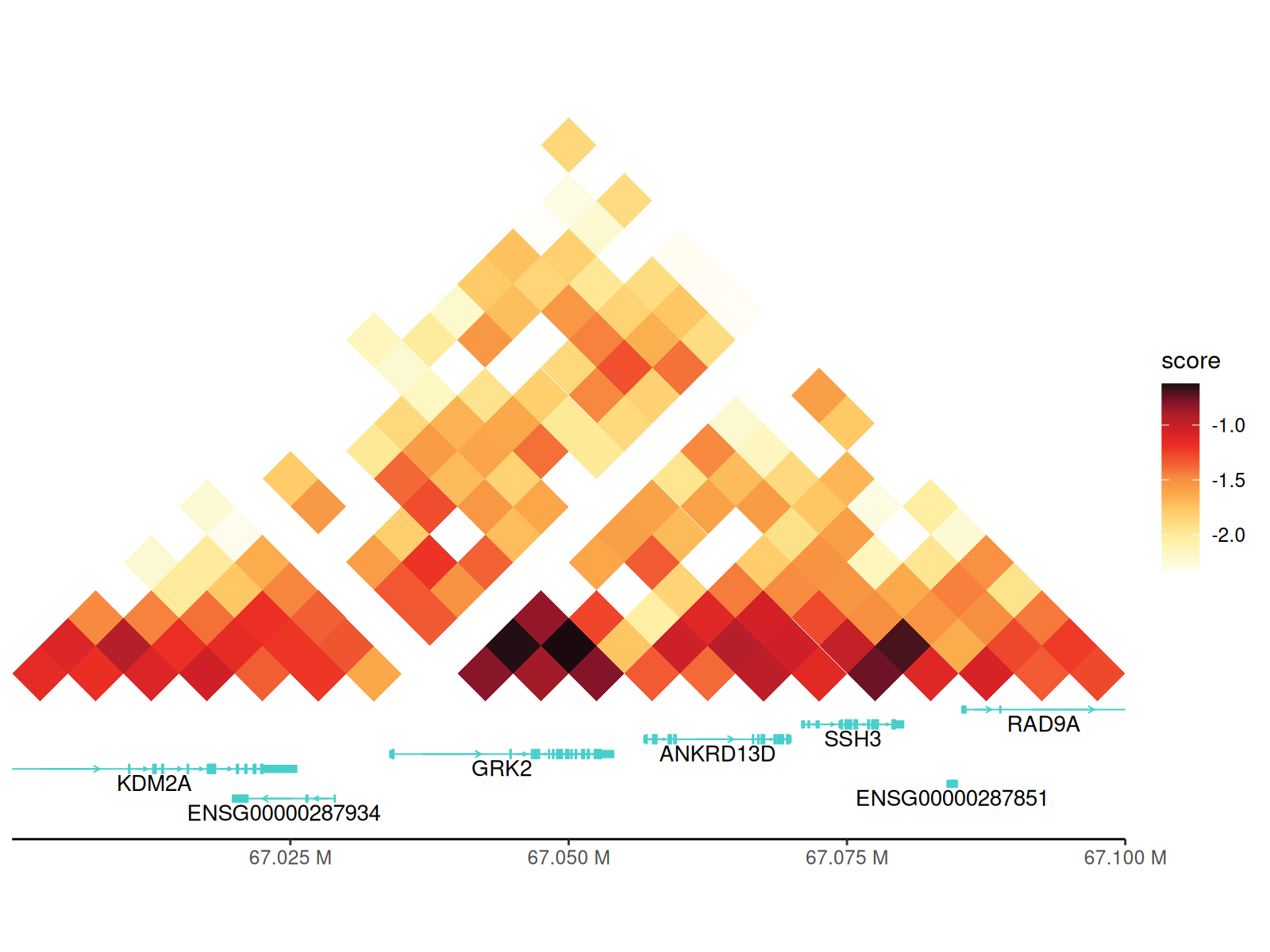

Hi-C visualization

Key parameters:

gtf_path: Path to GTF/GFF annotation file
style:
- "basic": Simple exon-intron structure
- "arrow": Adds directional arrows showing transcription direction
maxgap:
- Positive integer: Maximum gap between gene tracks (in bp)
- -1: Force all genes on single track (may overlap)
- 100000: Good default for most regions
gene_symbols: Character vector of specific genes to display (others hidden)
include_ncrna: Include non-coding RNAs (lncRNA, miRNA, etc.)

p + geom_annotation(
  gtf_path = path_gtf, style = "arrow", maxgap = -1,
  gene_symbols = c("GRK2", "SSH3", "KDM2A")
)

Hi-C visualization

Using the `annotation` Argument in `gghic()`

Again, you can also use the annotation argument in gghic() to add gene annotations directly.

cc_5["chr11:67000000-67100000"] |>
  gghic(
    ideogram = TRUE, genome = "hg19", highlight = FALSE, length_ratio = 0.7, ideogram_fontsize = 8,
    annotation = TRUE, gtf_path = path_gtf, style = "arrow", maxgap = -1, gene_symbols = c("GRK2", "SSH3", "KDM2A")
  )

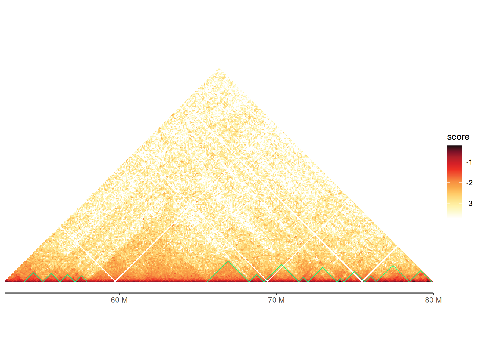
Adding TADs (Topologically Associating Domains)

TADs are visualized as triangles overlaid on the contact map, representing self-interacting genomic regions.

Visualization features: - Triangle apex points to TAD boundary - Triangle sides span the TAD region - Color and line style customizable - Automatically scaled to match heatmap coordinates

Two geoms available: - geom_tad(): Reads TAD file directly (convenient) - geom_tad2(): Uses data frame (more flexible for customization)

Using `tad` Argument in `gghic()`

cc_100["chr4:50000000-80000000"] |>
  gghic(
    tad = TRUE, tad_is_0based = TRUE, tad_path = path_tad,
    tad_colour = "#00ff83"
  )

Hi-C visualization

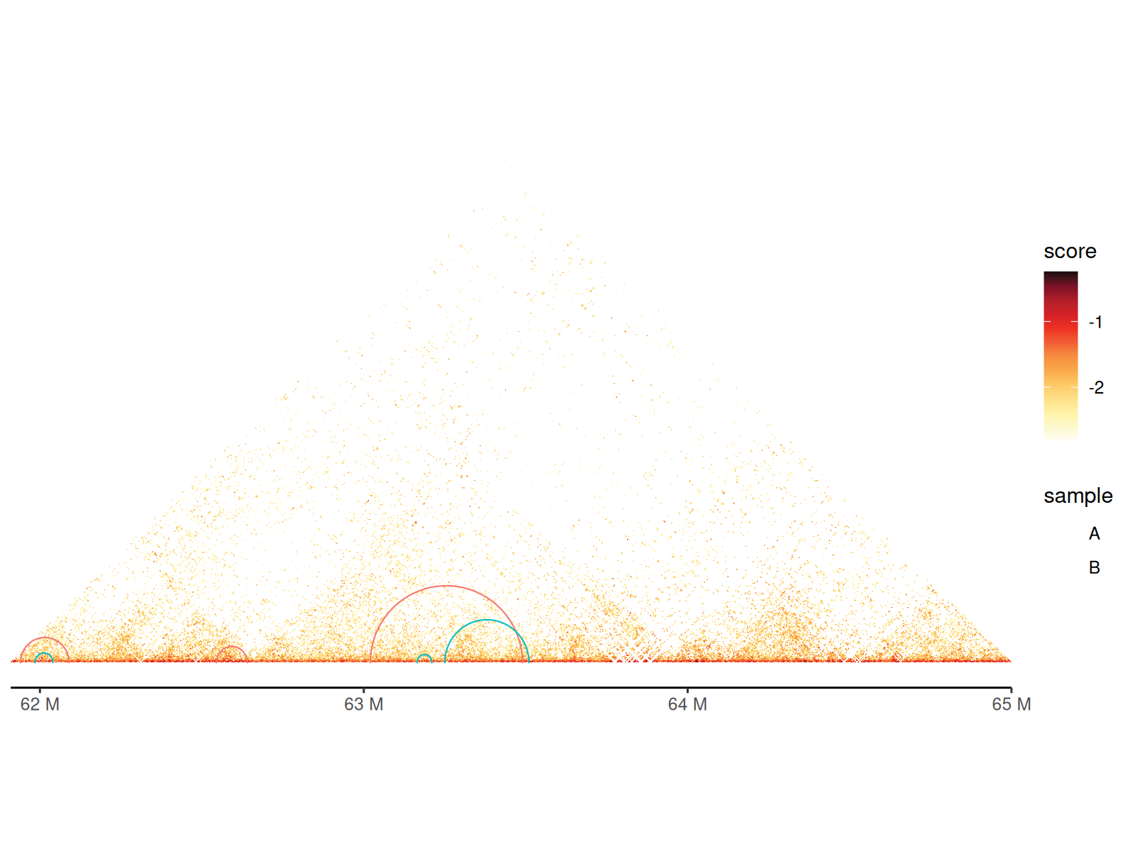
Using `geom_tad()` and `geom_tad2()`

Using geom_tad2() makes it easy to customize TAD aesthetics since you can provide a data.frame with additional columns.

df_tad <- path_tad |>
  read.table(
    sep = "\t", header = FALSE, col.names = c("seqnames", "start", "end")
  ) |>
  dplyr::mutate(start = start + 1) |>
  dplyr::filter(seqnames == "chr4", start > 60000000, end < 70000000) |>
  dplyr::mutate(sample = c("A", "B"))

df_100 |>
  dplyr::filter(
    seqnames1 == "chr4", seqnames2 == "chr4",
    start1 > 60000000, end1 < 70000000,
    start2 > 60000000, end2 < 70000000
  ) |>
  gghic(scale_column = "score", scale_method = function(x) x) +
  geom_tad2(
    data = df_tad, ggplot2::aes(
      seqnames = seqnames, start = start, end = end, colour = sample
    ), stroke = 2
  ) +
  ggplot2::scale_color_grey()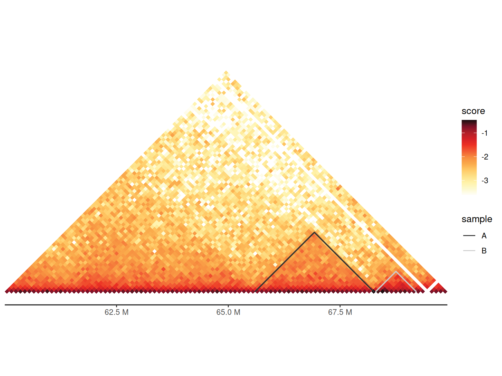

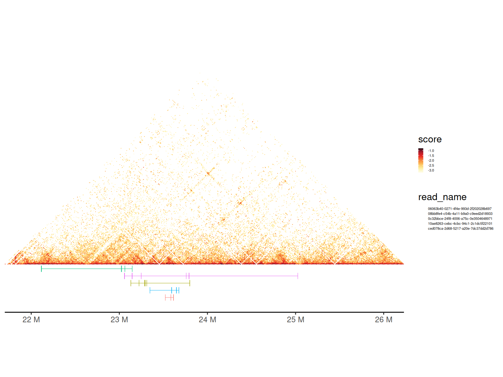
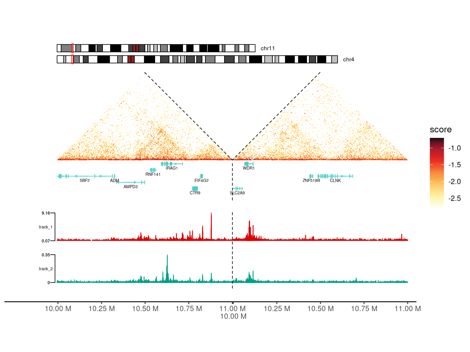
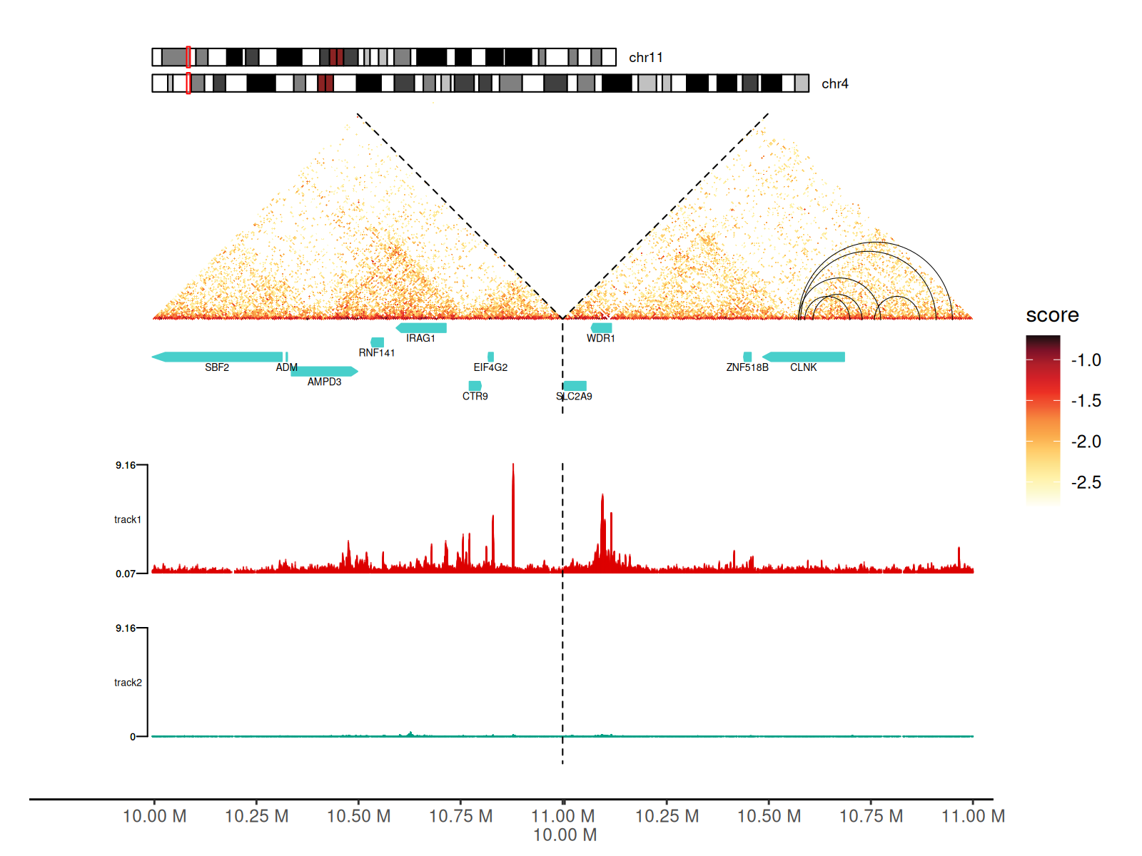
Hi-C visualization

Adding Chromatin Loops

Chromatin loops represent long-range interactions between specific genomic loci (e.g., enhancer-promoter contacts).

Visualization: - Drawn as arcs/semicircles connecting loop anchors - Arc height proportional to genomic distance - Customizable colors, line widths, and styles

Two geoms available: - geom_loop(): Reads BEDPE file directly - geom_loop2(): Uses data frame with custom aesthetics (color, size by significance)

Using `loop` Argument in `gghic()`

cc_5["chr11:61915000-65000000"] |>
  gghic(loop = TRUE)

Hi-C visualization

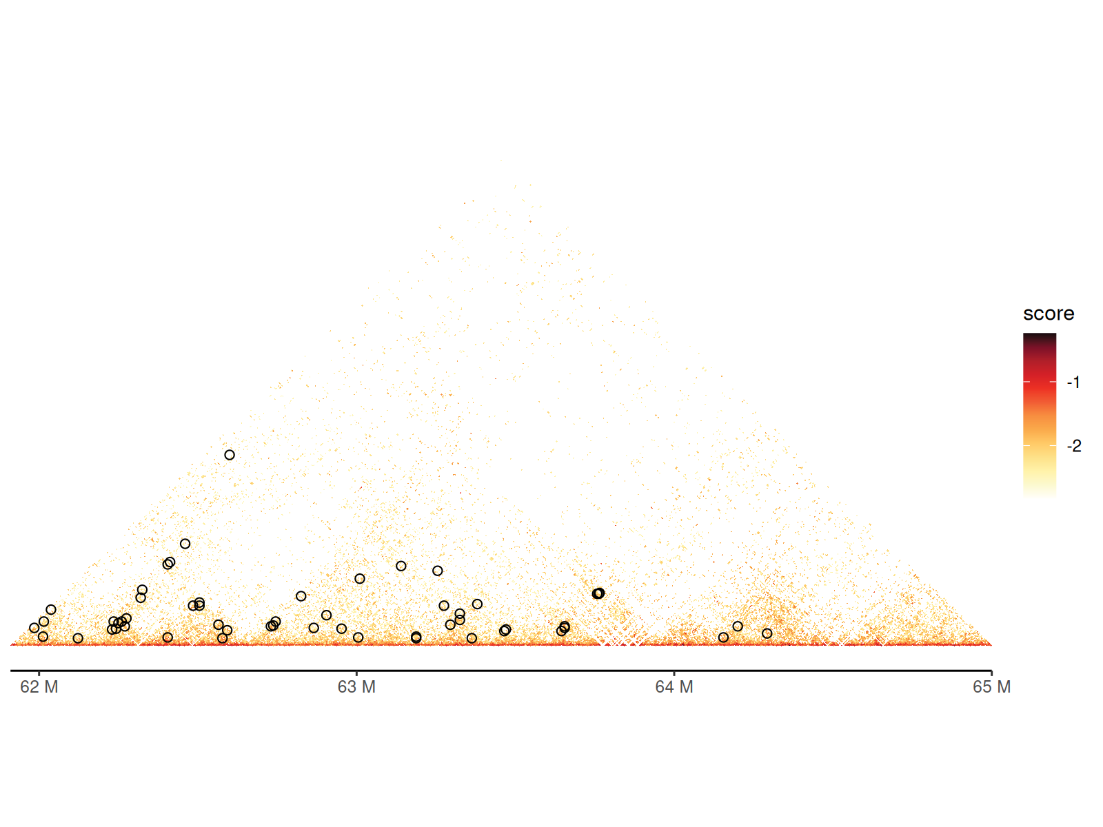
Using `geom_loop()` and `geom_loop2()`

Using geom_loop2() makes it easy to customize loop aesthetics since you can provide a data.frame with additional columns.

df_loop <- path_loop |>
  read.table(
    sep = "\t", col.names = c(
      "seqnames1", "start1", "end1", "seqnames2", "start2", "end2"
    )
  ) |>
  dplyr::filter(
    seqnames1 == "chr11", seqnames2 == "chr11",
    start1 > 61925000, end1 < 67480000,
    start2 > 61925000, end2 < 67480000
  )

keep <- sample(nrow(df_loop), 6)
df_loop <- df_loop |>
  dplyr::slice(keep) |>
  dplyr::mutate(
    sample = c(rep("A", 3), rep("B", 3))
  )

cc_5["chr11:61915000-65000000"] |>
  gghic() +
  geom_loop2(
    data = df_loop, ggplot2::aes(
      seqnames1 = seqnames1, start1 = start1, end1 = end1,
      seqnames2 = seqnames2, start2 = start2, end2 = end2, colour = sample
    ), stroke = 1, style = "arc"
  )

Hi-C visualization

Multi-Way Contact Visualization

Pore-C and similar technologies capture multi-way contacts where a single DNA molecule contacts 3+ genomic loci simultaneously.

What are concatemers? - Long DNA molecules captured by nanopore sequencing - Each molecule contains multiple chromatin contact points - Represented as sets of genomic intervals with a shared read ID

Visualization approach: - Each read shown as a colored horizontal bar - Bar width indicates genomic span of contacts - Overlaid on Hi-C heatmap for context

💡 See also: Hypergraph vignette for network-based analysis of multi-way contacts

Using `geom_concatemer()` and `geom_concatemer2()`

# Load the GInteractions object representing multi-way contacts
gis <- path_gis_hic |>
  readRDS()
df <- scaleData(gis, "balanced", log10)

# Select a few reads to visualize
names_read <- c(
  "0c32bbce-24f8-4006-a75c-0e3504648971",
  "10ae8263-cebc-4cbc-94c1-2c1dc5f22101",
  "ced078ca-2d68-5217-a20e-7dc37dd2d786",
  "06063b40-0271-4f4e-993d-2f202028b697",
  "08bb8fe4-c54b-4a11-b9a0-c9eed2d18933"
)
grs_concatemer <- path_concatemers |>
  readRDS() |>
  GenomicRanges::sort()
grs_concatemer <- grs_concatemer[
  GenomicRanges::seqnames(grs_concatemer) %in% c("chr22")
]
df_concatemers <- grs_concatemer |>
  tibble::as_tibble() |>
  dplyr::filter(read_name %in% names_read)

gghic(gis) +
  geom_concatemer2(
    data = df_concatemers, ggplot2::aes(
      seqnames = seqnames, start = start, end = end, read_group = read_name,
      colour = read_name
    ), check_concatemers = TRUE, width_ratio = 0.03
  ) +
  ggplot2::theme(
    legend.key.size = ggplot2::unit(2, "mm"),
    legend.text = ggplot2::element_text(size = 4)
  )

Hi-C visualization

Converting Concatemers to GInteractions

You can also generate a GInteractions object from a set of concatemers using concatemers2Gis() to visualize the contact frequency of the concatemers.

grs_concatemer_sub <- grs_concatemer[
  grs_concatemer$read_name %in% names_read
]

gis_concatemer <- concatemers2Gis(grs_concatemer_sub, bin_size = 100000)

gis_concatemer |>
  sort() |>
  tibble::as_tibble() |>
  dplyr::mutate(balanced = count) |>
  gghic(scale_method = function(x) x, ideogram = TRUE) +
  geom_concatemer2(
    data = df_concatemers,
    ggplot2::aes(
      seqnames = seqnames, start = start, end = end, read_group = read_name
    )
  ) +
  ggplot2::theme(
    legend.key.size = ggplot2::unit(2, "mm"),
    legend.text = ggplot2::element_text(size = 4)
  )

Hi-C visualization

Combining Heatmaps

You can combine two heatmaps using geom_hic_under() to visualize both pairwise interactions and multi-way contacts.

gghic(gis) +
  geom_concatemer2(
    data = df_concatemers,
    ggplot2::aes(
      seqnames = seqnames, start = start, end = end, read_group = read_name
    )
  ) +
  geom_hic_under(
    data = tibble::as_tibble(gis_concatemer) |> dplyr::mutate(score = count),
    ggplot2::aes(
      seqnames1 = seqnames1, start1 = start1, end1 = end1,
      seqnames2 = seqnames2, start2 = start2, end2 = end2, fill2 = score
    ), draw_boundary = FALSE
  ) |>
  renameGeomAes(new_aes = c("fill" = "fill2")) +
  scale_fill_viridis_c(
    aesthetics = "fill2", option = "A", guide = "legend", name = "count"
  )

Hi-C visualization

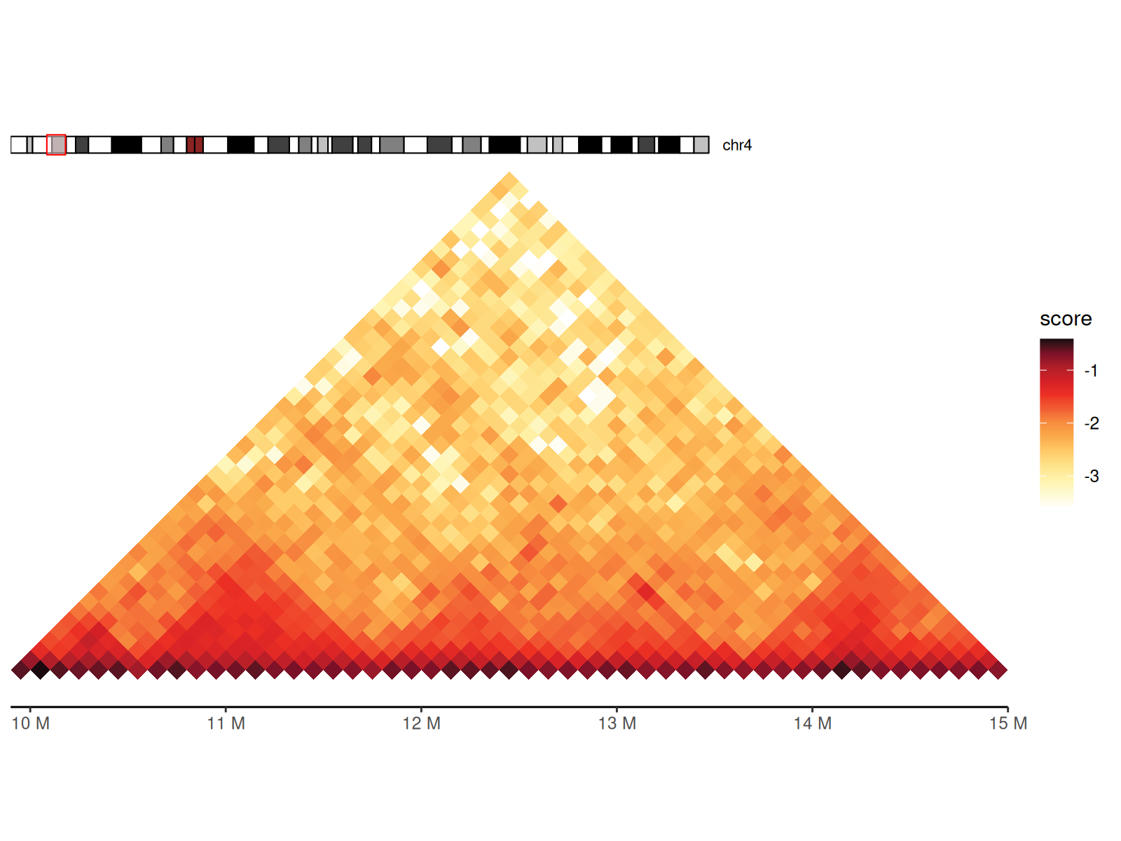
Multi-Chromosome Visualization

Visualize interactions across multiple chromosomes in a single unified plot.

Use cases: - Genome-wide interaction patterns - Trans-chromosomal contacts - Comparative Hi-C across chromosomes - Chromosome territory analysis

Layout features: - Each chromosome occupies a diagonal block - Inter-chromosomal interactions shown in off-diagonal blocks - Chromosome boundaries clearly demarcated

Key parameters: - draw_boundary = TRUE: Draws lines separating chromosomes - expand_xaxis = TRUE: Adds spacing between chromosomes for readability - expand_left: Additional left margin (in bp) when using ideograms/annotations

cc_100 |>
  gghic(draw_boundary = TRUE, expand_xaxis = TRUE)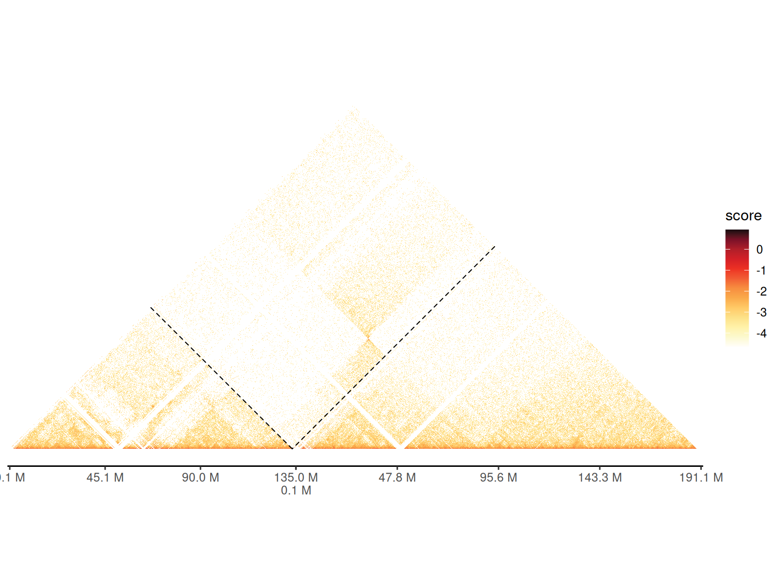

Hi-C visualization

Chromosome ideograms and gene tracks can also be added to the plot when visualizing multiple chromosomes.

p <- df_5 |>
  dplyr::filter(
    start1 > 10000000 & start1 < 11000000 &
      start2 > 10000000 & start2 < 11000000
  ) |>
  gghic(
    scale_column = "score", scale_method = function(x) x,
    ideogram = TRUE, genome = "hg19", highlight = TRUE, ideogram_fontsize = 7, ideogram_width_ratio = 0.08,
    annotation = TRUE, include_ncrna = FALSE, gtf_path = path_gtf, maxgap = 100000, annotation_fontsize = 5, annotation_width_ratio = 0.05,
    draw_boundary = TRUE, expand_xaxis = TRUE, expand_left = 300000
  )

p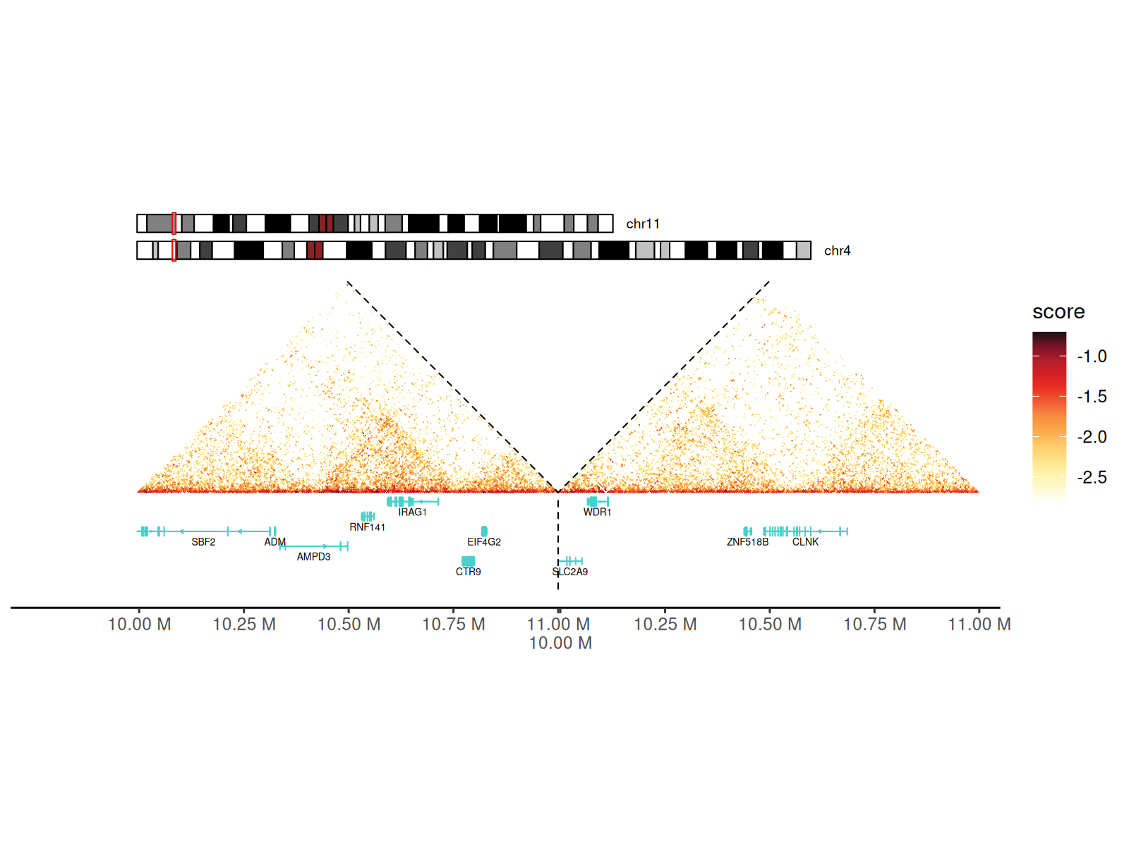

Hi-C visualization

Adding Signal Tracks

Integrate 1D genomic signals (ChIP-seq, ATAC-seq, RNA-seq, etc.) alongside Hi-C data.

Supported formats: - BigWig files (.bw, .bigWig) - Automatic data range detection or manual specification - Multiple tracks with independent colors and scales

Visualization: - Tracks displayed as area/mountain plots - Positioned on left side of heatmap - Aligned with genomic coordinates - Rasterization option for large datasets

Using `geom_track()` Layer

p + geom_track(
  data_paths = paths_track, width_ratio = 0.3, data_range = "auto",
  fill = c("#DC0000B2", "#00A087B2"), rasterize = TRUE
)

Hi-C visualization

Using `track` Argument in `gghic()`

gghic() is handy for adding all these features to the plot.

keep <- which(
  df_5$start1 > 10000000 & df_5$start1 < 11000000 &
    df_5$start2 > 10000000 & df_5$start2 < 11000000
)

cc_5[keep] |>
  gghic(
    draw_boundary = TRUE, rasterize = TRUE,
    ideogram = TRUE, genome = "hg19", highlight = TRUE, ideogram_fontsize = 7, ideogram_width_ratio = 0.08,
    annotation = TRUE, include_ncrna = FALSE, gtf_path = path_gtf,
    annotation_style = "arrow", maxgap = 100000, annotation_fontsize = 5, annotation_width_ratio = 0.05,
    track = TRUE, track_width_ratio = 0.5, track_fill = c("#DC0000B2", "#00A087B2"), data_range = "maximum",
    loop = TRUE, loop_style = "arc", stroke = 0.5,
    expand_xaxis = TRUE, expand_left = 300000
  )

Hi-C visualization

Session Information

sessionInfo()
#> R version 4.5.2 (2025-10-31)
#> Platform: x86_64-pc-linux-gnu
#> Running under: Ubuntu 24.04.3 LTS
#> 
#> Matrix products: default
#> BLAS:   /usr/lib/x86_64-linux-gnu/openblas-pthread/libblas.so.3 
#> LAPACK: /usr/lib/x86_64-linux-gnu/openblas-pthread/libopenblasp-r0.3.26.so;  LAPACK version 3.12.0
#> 
#> locale:
#>  [1] LC_CTYPE=C.UTF-8       LC_NUMERIC=C           LC_TIME=C.UTF-8       
#>  [4] LC_COLLATE=C.UTF-8     LC_MONETARY=C.UTF-8    LC_MESSAGES=C.UTF-8   
#>  [7] LC_PAPER=C.UTF-8       LC_NAME=C              LC_ADDRESS=C          
#> [10] LC_TELEPHONE=C         LC_MEASUREMENT=C.UTF-8 LC_IDENTIFICATION=C   
#> 
#> time zone: UTC
#> tzcode source: system (glibc)
#> 
#> attached base packages:
#> [1] stats4    stats     graphics  grDevices utils     datasets  methods  
#> [8] base     
#> 
#> other attached packages:
#>  [1] GenomicFeatures_1.62.0      AnnotationDbi_1.72.0       
#>  [3] gghic_0.2.1                 InteractionSet_1.38.0      
#>  [5] SummarizedExperiment_1.40.0 Biobase_2.70.0             
#>  [7] MatrixGenerics_1.22.0       matrixStats_1.5.0          
#>  [9] GenomicRanges_1.62.1        Seqinfo_1.0.0              
#> [11] IRanges_2.44.0              S4Vectors_0.48.0           
#> [13] BiocGenerics_0.56.0         generics_0.1.4             
#> [15] dplyr_1.1.4                 ggplot2_4.0.1              
#> 
#> loaded via a namespace (and not attached):
#>   [1] RColorBrewer_1.1-3       rstudioapi_0.18.0        jsonlite_2.0.0          
#>   [4] magrittr_2.0.4           farver_2.1.2             rmarkdown_2.30          
#>   [7] fs_1.6.6                 BiocIO_1.20.0            ragg_1.5.0              
#>  [10] vctrs_0.7.0              memoise_2.0.1            Rsamtools_2.26.0        
#>  [13] RCurl_1.98-1.17          base64enc_0.1-3          htmltools_0.5.9         
#>  [16] S4Arrays_1.10.1          progress_1.2.3           curl_7.0.0              
#>  [19] Rhdf5lib_1.32.0          SparseArray_1.10.8       Formula_1.2-5           
#>  [22] rhdf5_2.54.1             sass_0.4.10              bslib_0.9.0             
#>  [25] htmlwidgets_1.6.4        desc_1.4.3               Gviz_1.54.0             
#>  [28] httr2_1.2.2              cachem_1.1.0             GenomicAlignments_1.46.0
#>  [31] lifecycle_1.0.5          pkgconfig_2.0.3          Matrix_1.7-4            
#>  [34] R6_2.6.1                 fastmap_1.2.0            digest_0.6.39           
#>  [37] colorspace_2.1-2         textshaping_1.0.4        Hmisc_5.2-5             
#>  [40] RSQLite_2.4.5            filelock_1.0.3           labeling_0.4.3          
#>  [43] httr_1.4.7               abind_1.4-8              compiler_4.5.2          
#>  [46] bit64_4.6.0-1            withr_3.0.2              htmlTable_2.4.3         
#>  [49] S7_0.2.1                 backports_1.5.0          BiocParallel_1.44.0     
#>  [52] DBI_1.2.3                biomaRt_2.66.0           rappdirs_0.3.4          
#>  [55] DelayedArray_0.36.0      rjson_0.2.23             tools_4.5.2             
#>  [58] foreign_0.8-90           nnet_7.3-20              glue_1.8.0              
#>  [61] restfulr_0.0.16          rhdf5filters_1.22.0      grid_4.5.2              
#>  [64] checkmate_2.3.3          cluster_2.1.8.1          gtable_0.3.6            
#>  [67] BSgenome_1.78.0          tidyr_1.3.2              ensembldb_2.34.0        
#>  [70] data.table_1.18.0        hms_1.1.4                XVector_0.50.0          
#>  [73] pillar_1.11.1            stringr_1.6.0            BiocFileCache_3.0.0     
#>  [76] lattice_0.22-7           deldir_2.0-4             rtracklayer_1.70.1      
#>  [79] bit_4.6.0                biovizBase_1.58.0        tidyselect_1.2.1        
#>  [82] Biostrings_2.78.0        knitr_1.51               gridExtra_2.3           
#>  [85] ProtGenerics_1.42.0      xfun_0.56                stringi_1.8.7           
#>  [88] UCSC.utils_1.6.1         lazyeval_0.2.2           yaml_2.3.12             
#>  [91] evaluate_1.0.5           codetools_0.2-20         cigarillo_1.0.0         
#>  [94] interp_1.1-6             tibble_3.3.1             cli_3.6.5               
#>  [97] rpart_4.1.24             systemfonts_1.3.1        jquerylib_0.1.4         
#> [100] dichromat_2.0-0.1        Rcpp_1.1.1               GenomeInfoDb_1.46.2     
#> [103] dbplyr_2.5.1             png_0.1-8                XML_3.99-0.20           
#> [106] parallel_4.5.2           pkgdown_2.2.0            blob_1.3.0              
#> [109] prettyunits_1.2.0        jpeg_0.1-11              latticeExtra_0.6-31     
#> [112] AnnotationFilter_1.34.0  bitops_1.0-9             txdbmaker_1.6.2         
#> [115] viridisLite_0.4.2        VariantAnnotation_1.56.0 scales_1.4.0            
#> [118] purrr_1.2.1              crayon_1.5.3             rlang_1.1.7             
#> [121] KEGGREST_1.50.0

Minghao Jiang

2026-01-23

Introduction

Why gghic?

Key Features

Typical Workflow

Getting Started

Load Required Packages

Download Example data

Working with ChromatinContacts Objects

Understanding ChromatinContacts

Creating ChromatinContacts Objects

No Focus (Genome-Wide)

Focusing on Specific Regions

Single Region or Chromosome

Multiple Regions with Operators

Complex Focus Patterns

Using GInteractions Objects

Import Interaction Data

Adding Genomic Features

Manipulating ChromatinContacts Objects

Subsetting by Genomic Regions (character)

Subsetting with GRanges

Subsetting with GInteractions

Subsetting by Index or Logical Vector

Creating Visualizations

Visualization Approaches

1. High-Level Wrapper: gghic()

2. Low-Level Layers: geom_*()

Basic Hi-C Heatmap

Using geom_hic() Layer

Using gghic() Wrapper

Adding Chromosome Ideograms

Using geom_ideogram() Layer

Using the ideogram Argument in gghic()

Adding Gene Annotations

Using geom_annotation() Layer

Using the annotation Argument in gghic()

Adding TADs (Topologically Associating Domains)

Using tad Argument in gghic()

Using geom_tad() and geom_tad2()

Adding Chromatin Loops

Using loop Argument in gghic()

Using geom_loop() and geom_loop2()

Multi-Way Contact Visualization

Using geom_concatemer() and geom_concatemer2()

Converting Concatemers to GInteractions

Combining Heatmaps

Multi-Chromosome Visualization

Adding Signal Tracks

Using geom_track() Layer

Using track Argument in gghic()

Session Information

1. High-Level Wrapper: `gghic()`

2. Low-Level Layers: `geom_*()`

Using `geom_hic()` Layer

Using `gghic()` Wrapper

Using `geom_ideogram()` Layer

Using the `ideogram` Argument in `gghic()`

Using `geom_annotation()` Layer

Using the `annotation` Argument in `gghic()`

Using `tad` Argument in `gghic()`

Using `geom_tad()` and `geom_tad2()`

Using `loop` Argument in `gghic()`

Using `geom_loop()` and `geom_loop2()`

Using `geom_concatemer()` and `geom_concatemer2()`

Using `geom_track()` Layer

Using `track` Argument in `gghic()`