Multi-way Contact Analysis with Hypergraphs

Overview

Pore-C and similar long-read technologies capture multi-way chromatin contacts where a single DNA molecule can contact 3, 4, 5, or more genomic loci simultaneously. Traditional Hi-C analysis focuses on pairwise interactions, but multi-way contacts provide richer information about:

Higher-order chromatin structure: TAD hubs, chromatin loops involving multiple enhancers
Regulatory complexity: Multi-enhancer clusters coordinating gene expression
Phase separation: Condensate formation with many participants

This vignette shows how to analyze and visualize multi-way contacts using hypergraph representations with the MultiWayContacts S4 class, where:

Nodes (vertices) = Genomic bins
Hyperedges = Reads connecting multiple bins

Key Concepts

What is a Hypergraph?

A hypergraph is a generalization of a graph where edges (called hyperedges) can connect any number of vertices (nodes), not just two.

For chromatin contacts:

Pairwise contact (Hi-C): edge connecting 2 bins
3-way contact: hyperedge connecting 3 bins
N-way contact: hyperedge connecting N bins

Why Use Hypergraphs?

Traditional pairwise analysis loses information:

A read contacting bins {A, B, C, D} generates 6 pairwise contacts: AB, AC, AD, BC, BD, CD
But we can’t reconstruct which bins were contacted together on the same molecule
Hypergraphs preserve this simultaneity information

Filtering Strategy

Multi-way contact analysis requires careful filtering:

Bin contacts: Remove low-quality pairwise interactions (quantile filtering)
Multi-way degree: Keep only reads with ≥N contacts (e.g., ≥3)
Chromosome focus: Analyze specific chromosomes for clarity

Getting Started

Load required libraries:

load_pkg <- function(pkgs) {
  for (pkg in pkgs) suppressMessages(require(pkg, character.only = TRUE))
}

load_pkg(c("dplyr", "ggplot2", "gghic"))

Example Data Format

Your pairs file should be tab-separated with at least these columns:

read_name    chrom1  pos1  chrom2  pos2
read_001     chr1    1000  chr1    5000
read_001     chr1    1000  chr1    9000
read_002     chr2    2000  chr2    8000
...

Each row is a pairwise contact from a read. A read with 4 contacts generates 6 rows (all pairs).

Prepare Example Data

For this vignette, we’ll create synthetic Pore-C data and save it to a temporary file:

set.seed(42)

# Simulate multi-way contacts on multiple chromosomes
n_reads <- 500

# Chromosome information
chroms <- data.frame(
  chrom = c("chr21", "chr22"),
  length = c(46e6, 50e6), # 46 Mb and 50 Mb
  stringsAsFactors = FALSE
)

# Generate reads with varying numbers of contacts
read_data <- lapply(seq_len(n_reads), function(i) {
  read_name <- sprintf("read_%05d", i)

  # 20% chance of trans-chromosomal contacts
  is_trans <- runif(1) < 0.2

  if (is_trans) {
    # Trans-chromosomal: contacts on both chromosomes
    n_contacts_chr1 <- sample(2:4, 1)
    n_contacts_chr2 <- sample(2:4, 1)

    # Generate positions on chr21
    center1 <- runif(1, 10e6, chroms$length[1] - 10e6)
    spread1 <- runif(1, 1e6, 3e6)
    pos_chr1 <- sort(pmax(1, pmin(
      chroms$length[1],
      rnorm(n_contacts_chr1, center1, spread1)
    )))

    # Generate positions on chr22
    center2 <- runif(1, 10e6, chroms$length[2] - 10e6)
    spread2 <- runif(1, 1e6, 3e6)
    pos_chr2 <- sort(pmax(1, pmin(
      chroms$length[2],
      rnorm(n_contacts_chr2, center2, spread2)
    )))

    # Create all pairwise combinations
    all_positions <- list(
      chr1 = data.frame(chrom = chroms$chrom[1], pos = as.integer(pos_chr1)),
      chr2 = data.frame(chrom = chroms$chrom[2], pos = as.integer(pos_chr2))
    )

    all_contacts <- rbind(all_positions$chr1, all_positions$chr2)
    n_total <- nrow(all_contacts)

    if (n_total < 2) {
      return(NULL)
    }

    pairs_list <- combn(n_total, 2, simplify = FALSE)

    do.call(rbind, lapply(pairs_list, function(pair) {
      data.frame(
        read_name = read_name,
        chrom1 = all_contacts$chrom[pair[1]],
        pos1 = all_contacts$pos[pair[1]],
        chrom2 = all_contacts$chrom[pair[2]],
        pos2 = all_contacts$pos[pair[2]],
        stringsAsFactors = FALSE
      )
    }))
  } else {
    # Intra-chromosomal: contacts on single chromosome
    chr_idx <- sample(1:2, 1, prob = c(0.3, 0.7))
    chr <- chroms$chrom[chr_idx]
    chr_length <- chroms$length[chr_idx]

    n_contacts <- sample(3:8, 1, prob = c(0.3, 0.25, 0.2, 0.15, 0.07, 0.03))

    center <- runif(1, 10e6, chr_length - 10e6)
    spread <- runif(1, 1e6, 5e6)
    positions <- sort(pmax(1, pmin(
      chr_length,
      rnorm(n_contacts, center, spread)
    )))

    if (n_contacts < 2) {
      return(NULL)
    }

    pairs <- combn(n_contacts, 2, simplify = FALSE)

    do.call(rbind, lapply(pairs, function(pair) {
      data.frame(
        read_name = read_name,
        chrom1 = chr,
        pos1 = as.integer(positions[pair[1]]),
        chrom2 = chr,
        pos2 = as.integer(positions[pair[2]]),
        stringsAsFactors = FALSE
      )
    }))
  }
})

pairs_df <- do.call(rbind, read_data)

# Add some noise
noise_pairs <- do.call(rbind, lapply(1:100, function(i) {
  chr <- sample(chroms$chrom, 1)
  chr_length <- chroms$length[chroms$chrom == chr]
  data.frame(
    read_name = sprintf("noise_%04d", i),
    chrom1 = chr,
    pos1 = sample(1:chr_length, 1),
    chrom2 = chr,
    pos2 = sample(1:chr_length, 1),
    stringsAsFactors = FALSE
  )
}))

pairs_df <- rbind(pairs_df, noise_pairs)

# Save to temporary file
pairs_file <- tempfile(fileext = ".pairs.gz")
gz <- gzfile(pairs_file, "w")
write.table(pairs_df, gz, sep = "\t", quote = FALSE, row.names = FALSE)
close(gz)

# Summary
cat(sprintf(
  "Generated %d pairwise contacts from %d reads\n",
  nrow(pairs_df), length(unique(pairs_df$read_name))
))
#> Generated 5319 pairwise contacts from 600 reads

trans_contacts <- sum(pairs_df$chrom1 != pairs_df$chrom2)
cat(sprintf(
  "  Intra-chromosomal: %d (%.1f%%)\n",
  nrow(pairs_df) - trans_contacts,
  100 * (nrow(pairs_df) - trans_contacts) / nrow(pairs_df)
))
#>   Intra-chromosomal: 4438 (83.4%)
cat(sprintf(
  "  Trans-chromosomal: %d (%.1f%%)\n",
  trans_contacts, 100 * trans_contacts / nrow(pairs_df)
))
#>   Trans-chromosomal: 881 (16.6%)

head(pairs_df, 10)
#>     read_name chrom1     pos1 chrom2     pos2
#> 1  read_00001  chr21 27651551  chr21 31762442
#> 2  read_00001  chr21 27651551  chr21 33514326
#> 3  read_00001  chr21 31762442  chr21 33514326
#> 4  read_00002  chr21 21721090  chr21 28230868
#> 5  read_00002  chr21 21721090  chr21 31627427
#> 6  read_00002  chr21 28230868  chr21 31627427
#> 7  read_00003  chr21 25627609  chr21 25874411
#> 8  read_00003  chr21 25627609  chr21 26736871
#> 9  read_00003  chr21 25874411  chr21 26736871
#> 10 read_00004  chr22  6959097  chr22  9658680

Workflow with MultiWayContacts

The MultiWayContacts S4 class provides a streamlined, object-oriented workflow for analyzing multi-way contacts. The typical analysis follows these steps:

Create MultiWayContacts object
Import pairs data
Build hypergraph
Tidy to long format
Select top hyperedges
Visualize with gghypergraph()

Single Chromosome Analysis

# Create MultiWayContacts object for chr22
mc_chr22 <- MultiWayContacts(pairs_path = pairs_file, focus = "chr22")

# Complete workflow using pipes
mc_chr22 <- mc_chr22 |>
  import() |> # Load pairs data
  build(
    bin_size = 500000L, # 500 Kb bins
    quantile = 0.80, # Top 20% contacts
    min_multiway = 3
  ) |> # ≥3-way contacts
  gghic::tidy() |> # Convert to long format
  gghic::select(n_intra = 10) # Select top hyperedges
#> Reading pairs from file using C implementation...
#> Reading pairs from: /tmp/RtmpyIYAmV/file1eb635ace9d3.pairs.gz
#> Filtering for chromosome: chr22
#> Mode: (intra-chromosomal only)
#> 
#> Total: 5320 lines processed, 2779 contacts retained
#> Processing 2,779 contacts (chr22)
#> Removed 471 duplicate pairwise contacts within reads (2,308 remaining)
#> Filtering bin pairs with >= 3 contacts (80% quantile)
#> Retained 1,337 contacts from 341 reads
#> Estimated matrix size: 0.0 GB, Available RAM: 12.6 GB (threshold: 10.1 GB)
#> Identifying unique hyperedge patterns...
#> Removed 14 duplicate hyperedges (327 unique patterns)
#> Final hypergraph: 68 bins, 238 unique hyperedges (min 3-way contacts)

# Visualize
gghypergraph(mc_chr22, color_by = "n_multiways", palette = "viridis")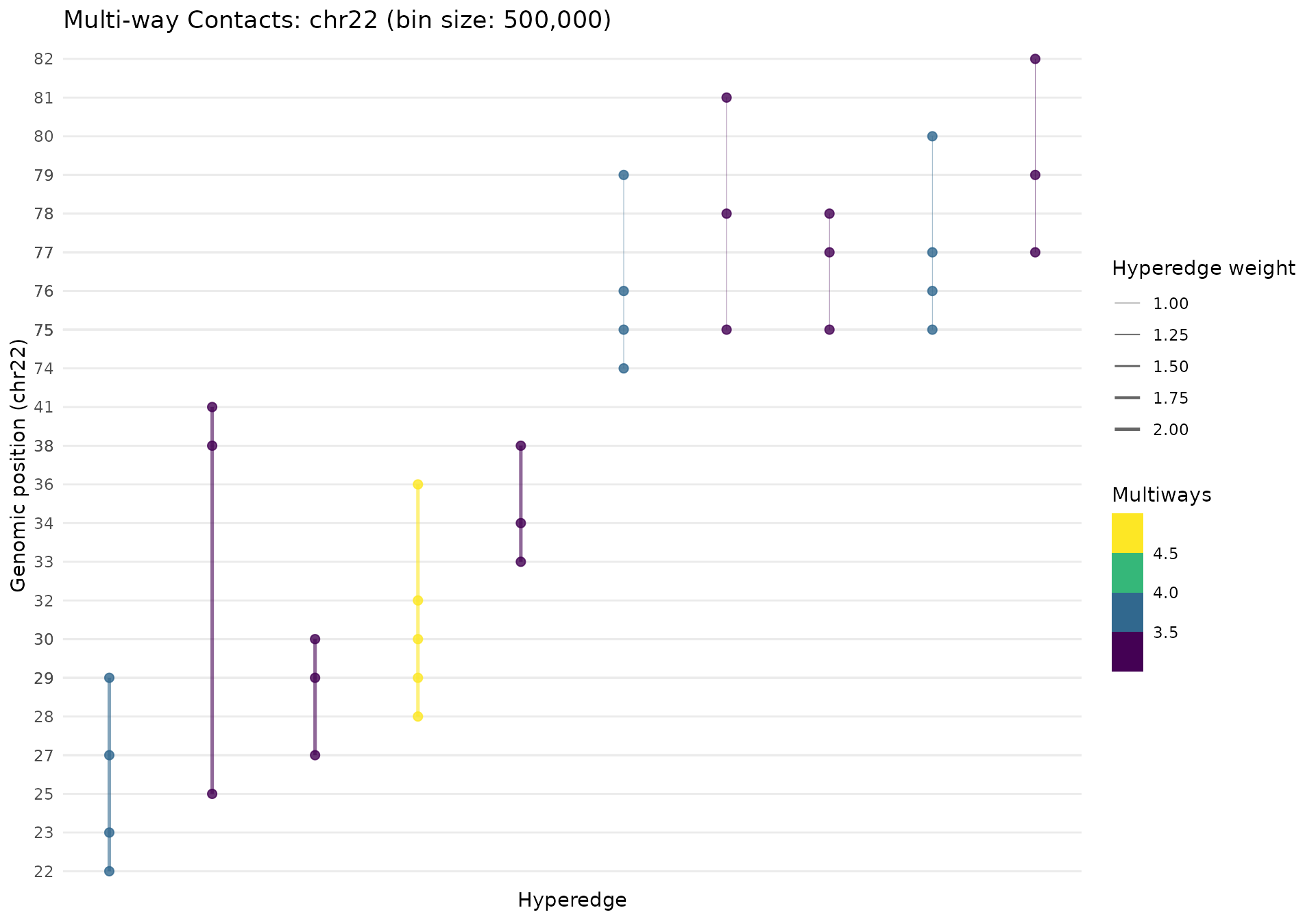

Hypergraph visualization

Multiple Chromosomes

# Analyze both chr21 and chr22
mc_multi <- MultiWayContacts(
  pairs_path = pairs_file, focus = c("chr21", "chr22")
)

mc_multi <- mc_multi |>
  import(inter_chrom = TRUE) |>
  build(bin_size = 500000L, quantile = 0.80, min_multiway = 3) |>
  gghic::tidy() |>
  gghic::select(n_intra = 10, n_inter = 10)
#> Reading pairs from file using C implementation...
#> Reading pairs from: /tmp/RtmpyIYAmV/file1eb635ace9d3.pairs.gz
#> Filtering for 2 chromosomes
#> Mode: (intra- and inter-chromosomal)
#> 
#> Total: 5320 lines processed, 5319 contacts retained
#> Processing 5,319 contacts (2 chromosomes)
#> Removed 872 duplicate pairwise contacts within reads (4,447 remaining)
#> Filtering bin pairs with >= 2 contacts (80% quantile)
#> Retained 2,873 contacts from 496 reads
#> Estimated matrix size: 0.0 GB, Available RAM: 12.6 GB (threshold: 10.0 GB)
#> Identifying unique hyperedge patterns...
#> Removed 3 duplicate hyperedges (493 unique patterns)
#> Final hypergraph: 138 bins, 435 unique hyperedges (min 3-way contacts)

# Faceted view (separate panels per chromosome)
gghypergraph(mc_multi, facet_chrom = FALSE)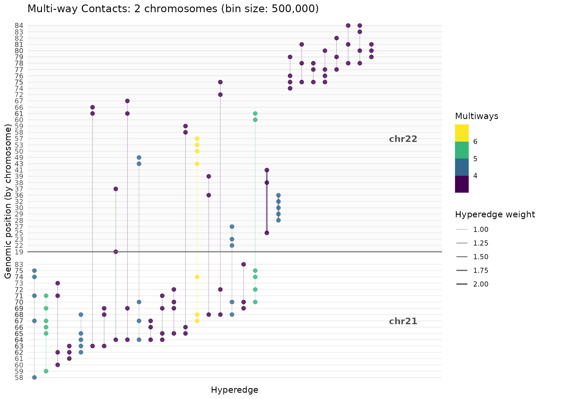

Hypergraph visualization

Method Details

import()

Loads pairs data from file. The data can be filtered to:

Specific chromosome(s) (via focus parameter in constructor)
Intra-chromosomal only (default) or include inter-chromosomal (inter_chrom = TRUE)

# Intra-chromosomal only (default)
mc <- MultiWayContacts(pairs_path) |>
  import()

# Include inter-chromosomal
mc <- MultiWayContacts(pairs_path) |>
  import(inter_chrom = TRUE)

build()

Constructs the hypergraph through several steps:

Binning: Aggregate contacts into genomic bins
Filtering: Remove low-frequency bin pairs (by quantile threshold)
Incidence matrix: Build sparse matrix (bins × reads)
Deduplication: Merge identical hyperedge patterns
Multiway filtering: Keep only hyperedges with ≥ min_multiway contacts

Parameters:

bin_size: Genomic bin size (default 1 Mb). Smaller = higher resolution but sparser
quantile: Threshold for bin pair filtering (default 0.85). Higher = more stringent
min_multiway: Minimum contacts per hyperedge (default 2)

# High resolution, strict filtering
mc |>
  build(bin_size = 100000L, quantile = 0.90, min_multiway = 4)

# Lower resolution, permissive filtering
mc |>
  build(bin_size = 1000000L, quantile = 0.75, min_multiway = 2)

tidy()

Converts the sparse incidence matrix to a tidy long-format data frame.

Parameters:

max_hyperedges: Subset to top N hyperedges by contact order (default: all)
weight_normalization: Weight transformation:
- "none": Raw frequency counts (default)
- "log": Log-transformed
- "by_order": Normalized within each contact order
- "minmax": Scaled to [0, 1]

# Top 50 hyperedges with log weights
mc |>
  tidy(max_hyperedges = 50, weight_normalization = "log")

# All hyperedges with normalized weights
mc |>
  tidy(weight_normalization = "by_order")

select()

Selects top-weighted hyperedges for visualization. For each chromosome, selects:

Top n_intra intra-chromosomal hyperedges
Top n_inter inter-chromosomal hyperedges

If fewer intra-chromosomal hyperedges exist, the remaining quota is added to inter-chromosomal selection.

Parameters:

n_intra: Number of intra-chromosomal hyperedges per chromosome (default 5)
n_inter: Number of inter-chromosomal hyperedges per chromosome (default 5)
n_multiways_filter: Keep only specific contact orders (e.g., c(3, 4))
chroms: Focus on specific chromosome(s)
append: Add to existing selection (TRUE) or replace (FALSE)

# Select more hyperedges
mc |>
  gghic::select(n_intra = 15, n_inter = 10)

# Only 3-way and 4-way contacts
mc |>
  gghic::select(n_multiways_filter = c(3, 4))

# Focus on chr1
mc |>
  gghic::select(chroms = "chr1", append = FALSE)

# Accumulate selections
mc |>
  gghic::select(chroms = "chr1", append = FALSE) |>
  gghic::select(chroms = "chr2", append = TRUE)

gghypergraph()

Creates a ggplot2 visualization of selected hyperedges.

Parameters:

point_size: Size of bin points (default 2)
line_width: Base width of hyperedge lines (default 0.3)
line_alpha: Transparency of lines (default 0.6)
color_by: Variable for coloring ("n_multiways" or other)
palette: Color palette ("viridis", "magma", "plasma", etc.)
facet_chrom: Separate panels per chromosome (TRUE) or composite y-axis (FALSE)

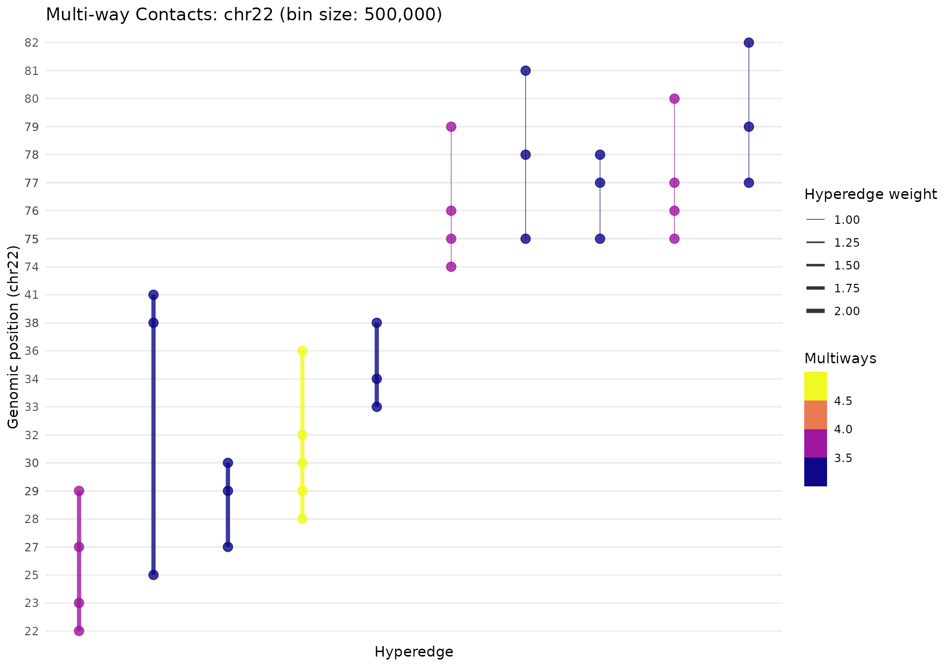
gghypergraph(
  mc_chr22,
  point_size = 3,
  line_width = 0.5,
  line_alpha = 0.8,
  palette = "plasma",
  facet_chrom = TRUE
)

Hypergraph visualization

The plot shows:

X-axis: Hyperedges (sorted by genomic position)
Y-axis: Genomic bins (position within chromosome)
Line width: Scales with hyperedge weight
Line color: By contact order (number of bins)

Other Examples

Filtering by Contact Order

# Focus on high-order contacts only (≥5-way)
mc_high_order <- MultiWayContacts(pairs_file, focus = "chr22") |>
  import() |>
  build(bin_size = 500000L, quantile = 0.85, min_multiway = 5) |>
  gghic::tidy() |>
  gghic::select(n_intra = 10, n_inter = 0)
#> Reading pairs from file using C implementation...
#> Reading pairs from: /tmp/RtmpyIYAmV/file1eb635ace9d3.pairs.gz
#> Filtering for chromosome: chr22
#> Mode: (intra-chromosomal only)
#> 
#> Total: 5320 lines processed, 2779 contacts retained
#> Processing 2,779 contacts (chr22)
#> Removed 471 duplicate pairwise contacts within reads (2,308 remaining)
#> Filtering bin pairs with >= 4 contacts (85% quantile)
#> Retained 860 contacts from 301 reads
#> Estimated matrix size: 0.0 GB, Available RAM: 12.5 GB (threshold: 10.0 GB)
#> Identifying unique hyperedge patterns...
#> Removed 36 duplicate hyperedges (265 unique patterns)
#> Final hypergraph: 60 bins, 46 unique hyperedges (min 5-way contacts)

gghypergraph(mc_high_order, palette = "inferno")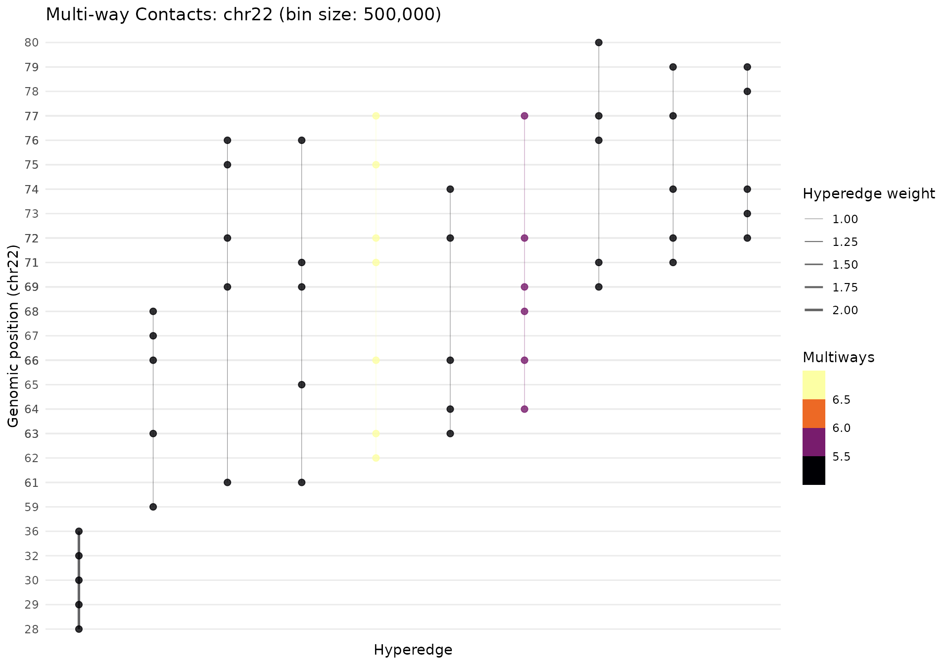

Hypergraph visualization

Comparing Chromosomes

# Select from both chromosomes independently
mc_compare <- MultiWayContacts(pairs_file, focus = c("chr21", "chr22")) |>
  import() |>
  build(bin_size = 500000L) |>
  gghic::tidy() |>
  gghic::select(n_intra = 10, n_inter = 5, append = FALSE)
#> Reading pairs from file using C implementation...
#> Reading pairs from: /tmp/RtmpyIYAmV/file1eb635ace9d3.pairs.gz
#> Filtering for 2 chromosomes
#> Mode: (intra-chromosomal only)
#> 
#> Total: 5320 lines processed, 4438 contacts retained
#> Processing 4,438 contacts (2 chromosomes)
#> Removed 97 reads with inter-chromosomal contacts (503 reads remaining)
#> Removed 649 duplicate pairwise contacts within reads (3,140 remaining)
#> Filtering bin pairs with >= 3 contacts (85% quantile)
#> Retained 1,290 contacts from 353 reads
#> Estimated matrix size: 0.0 GB, Available RAM: 12.3 GB (threshold: 9.9 GB)
#> Identifying unique hyperedge patterns...
#> Removed 18 duplicate hyperedges (335 unique patterns)
#> Final hypergraph: 112 bins, 331 unique hyperedges (min 2-way contacts)

# Faceted comparison
gghypergraph(mc_compare, facet_chrom = TRUE)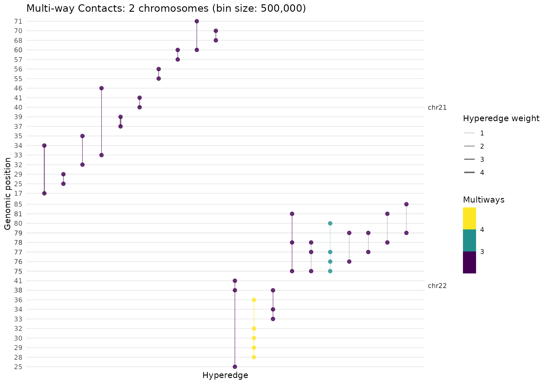

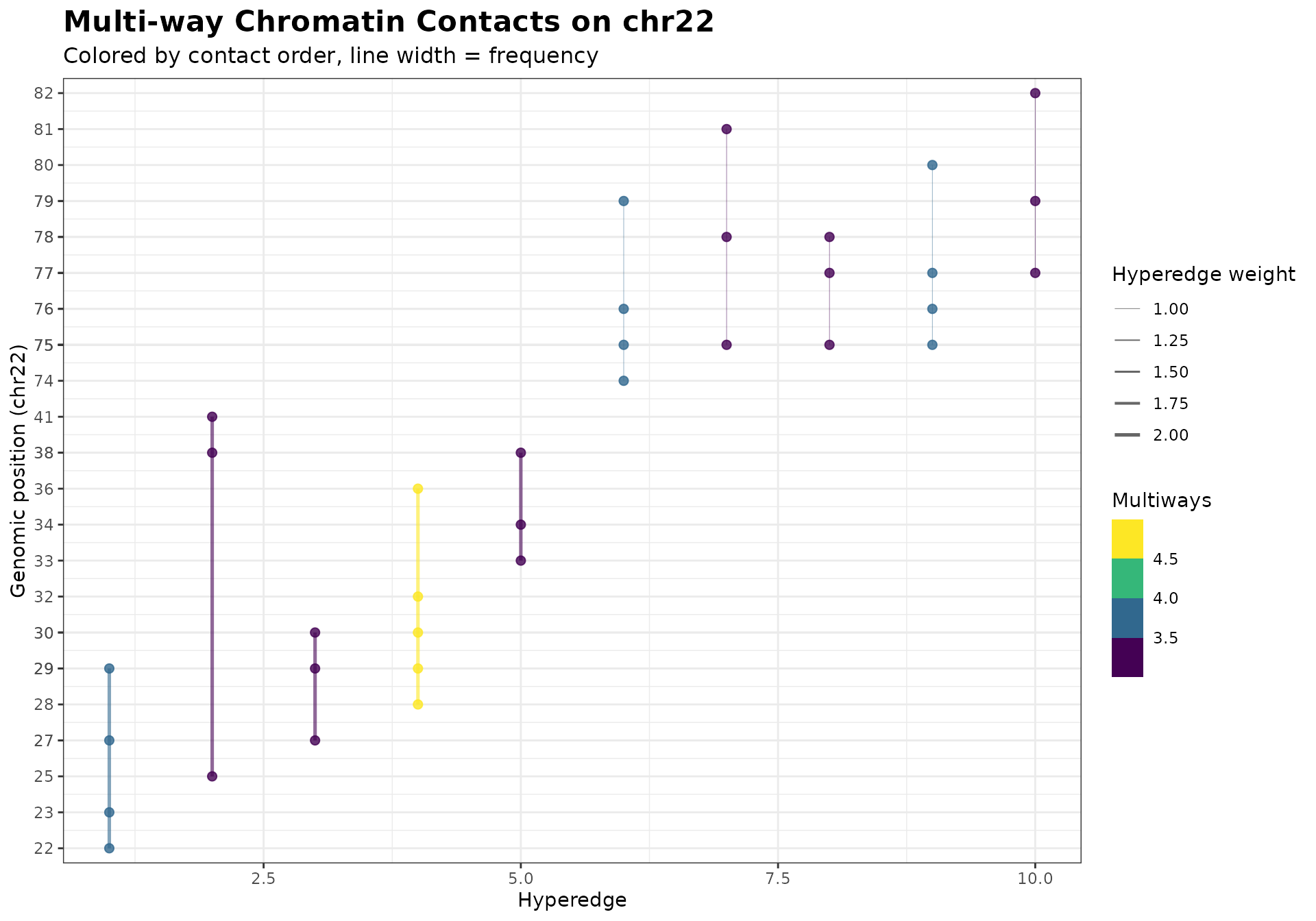
Hypergraph visualization

Customizing Plots

# Get base plot and customize
p <- gghypergraph(mc_chr22, facet_chrom = FALSE)

# Add custom styling
p +
  ggplot2::theme_bw() +
  ggplot2::labs(
    title = "Multi-way Chromatin Contacts on chr22",
    subtitle = "Colored by contact order, line width = frequency"
  ) +
  ggplot2::theme(
    plot.title = element_text(size = 16, face = "bold"),
    plot.subtitle = element_text(size = 12)
  )

Hypergraph visualization

Interpreting Results

Contact Order Distribution

# Examine distribution of contact orders
if (!is.null(hypergraphData(mc_multi, "selected"))) {
  contact_summary <- hypergraphData(mc_multi, "selected") |>
    dplyr::distinct(hyperedge_idx, n_multiways) |>
    dplyr::count(n_multiways, name = "n_hyperedges")

  print(contact_summary)

  ggplot2::ggplot(
    contact_summary,
    ggplot2::aes(x = n_multiways, y = n_hyperedges)
  ) +
    ggplot2::geom_col(fill = "steelblue") +
    ggplot2::labs(
      x = "Number of contacts (multiway order)",
      y = "Number of hyperedges",
      title = "Distribution of Contact Orders"
    ) +
    ggplot2::theme_minimal()
}
#> # A tibble: 5 × 2
#>   n_multiways n_hyperedges
#>         <dbl>        <int>
#> 1           3           13
#> 2           4            9
#> 3           5            5
#> 4           6            2
#> 5           7            1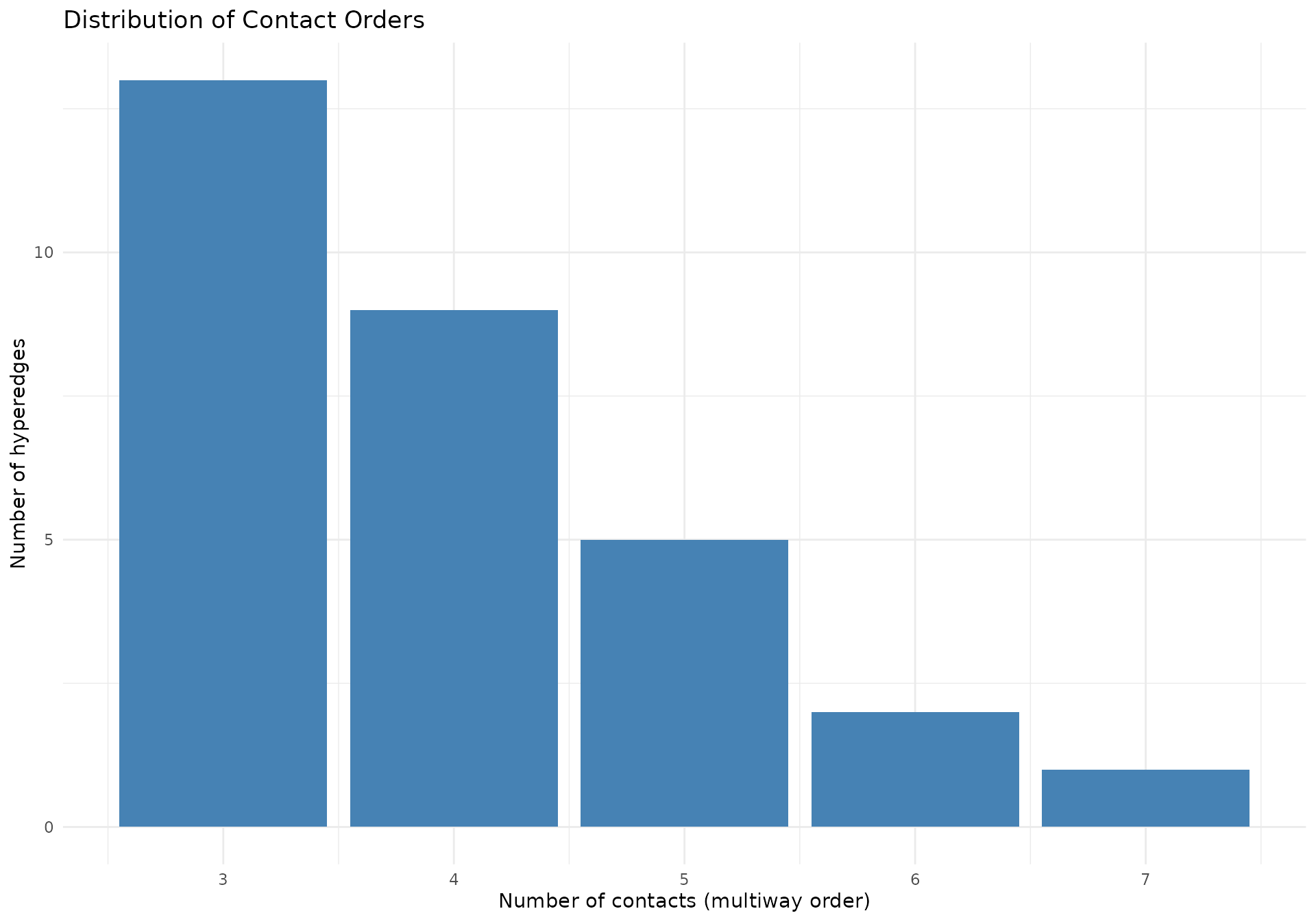

Hypergraph visualization

Intra vs Inter-chromosomal

# Check balance of intra vs inter contacts
if (!is.null(hypergraphData(mc_multi, "selected"))) {
  type_summary <- hypergraphData(mc_multi, "selected") |>
    dplyr::distinct(hyperedge_idx, type) |>
    dplyr::count(type)

  print(type_summary)
}
#> # A tibble: 2 × 2
#>   type      n
#>   <chr> <int>
#> 1 inter    10
#> 2 intra    20

Best Practices

Start with single chromosome: Easier to interpret and faster to compute
Tune bin size: Use resolution_depth vignette to find optimal resolution
Adjust quantile:

Higher (0.9-0.95): Very strict, fewer but high-confidence contacts
Lower (0.75-0.85): More permissive, capture weaker signals

Filter by multiway order: Focus on specific contact orders for targeted analysis
Use composite view (facet_chrom = FALSE) for multi-chromosome to see relationships
Weight normalization: Use "by_order" to compare across different contact orders fairly

Using geom_hypergraph for Custom Plots

While gghypergraph() provides a convenient high-level interface, you can also use geom_hypergraph() directly for more customization. This is useful when you want to:

Combine hypergraph with other ggplot2 layers
Create custom faceting or layouts
Apply custom themes and styling
Build complex multi-panel figures

Basic Usage

# Extract the selected hypergraph data
df <- hypergraphData(mc_chr22, "selected")

# Create custom x-axis ordering (by genomic position)
hyperedge_order <- df |>
  dplyr::mutate(chrom_num = as.numeric(gsub("\\D", "", chrom))) |>
  dplyr::group_by(hyperedge_idx) |>
  dplyr::summarise(
    min_chrom_num = min(chrom_num, na.rm = TRUE),
    min_bin = min(bin),
    .groups = "drop"
  ) |>
  dplyr::arrange(min_chrom_num, min_bin) |>
  dplyr::pull(hyperedge_idx)

df <- df |>
  dplyr::mutate(
    x = as.numeric(factor(hyperedge_idx, levels = hyperedge_order)),
    y = bin
  )

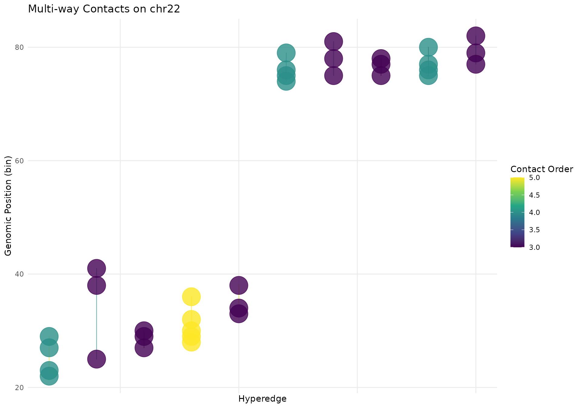
# Create plot with geom_hypergraph
ggplot2::ggplot(df, ggplot2::aes(x = x, y = y, group = hyperedge_idx)) +
  geom_hypergraph(
    ggplot2::aes(colour = n_multiways),
    line_width = 0.4,
    line_alpha = 0.7,
    point_size = 2.5
  ) +
  ggplot2::scale_color_viridis_c(name = "Contact Order") +
  ggplot2::labs(
    title = "Multi-way Contacts on chr22",
    x = "Hyperedge",
    y = "Genomic Position (bin)"
  ) +
  ggplot2::theme_minimal() +
  ggplot2::theme(
    panel.grid.minor = ggplot2::element_blank(),
    axis.text.x = ggplot2::element_blank(),
    axis.ticks.x = ggplot2::element_blank()
  )

Hypergraph visualization

Multi-Chromosome with Custom Layout

# Get multi-chromosome data
df_multi <- hypergraphData(mc_multi, "selected")

# Order hyperedges
hyperedge_order_multi <- df_multi |>
  dplyr::mutate(chrom_num = as.numeric(gsub("\\D", "", chrom))) |>
  dplyr::group_by(hyperedge_idx) |>
  dplyr::summarise(
    min_chrom_num = min(chrom_num, na.rm = TRUE),
    min_chrom = dplyr::first(chrom[chrom_num == min_chrom_num]),
    min_bin = min(bin[chrom == min_chrom]),
    .groups = "drop"
  ) |>
  dplyr::arrange(min_chrom_num, min_bin) |>
  dplyr::pull(hyperedge_idx)

df_multi <- df_multi |>
  dplyr::mutate(
    x = as.numeric(factor(hyperedge_idx, levels = hyperedge_order_multi))
  )

# Create faceted plot
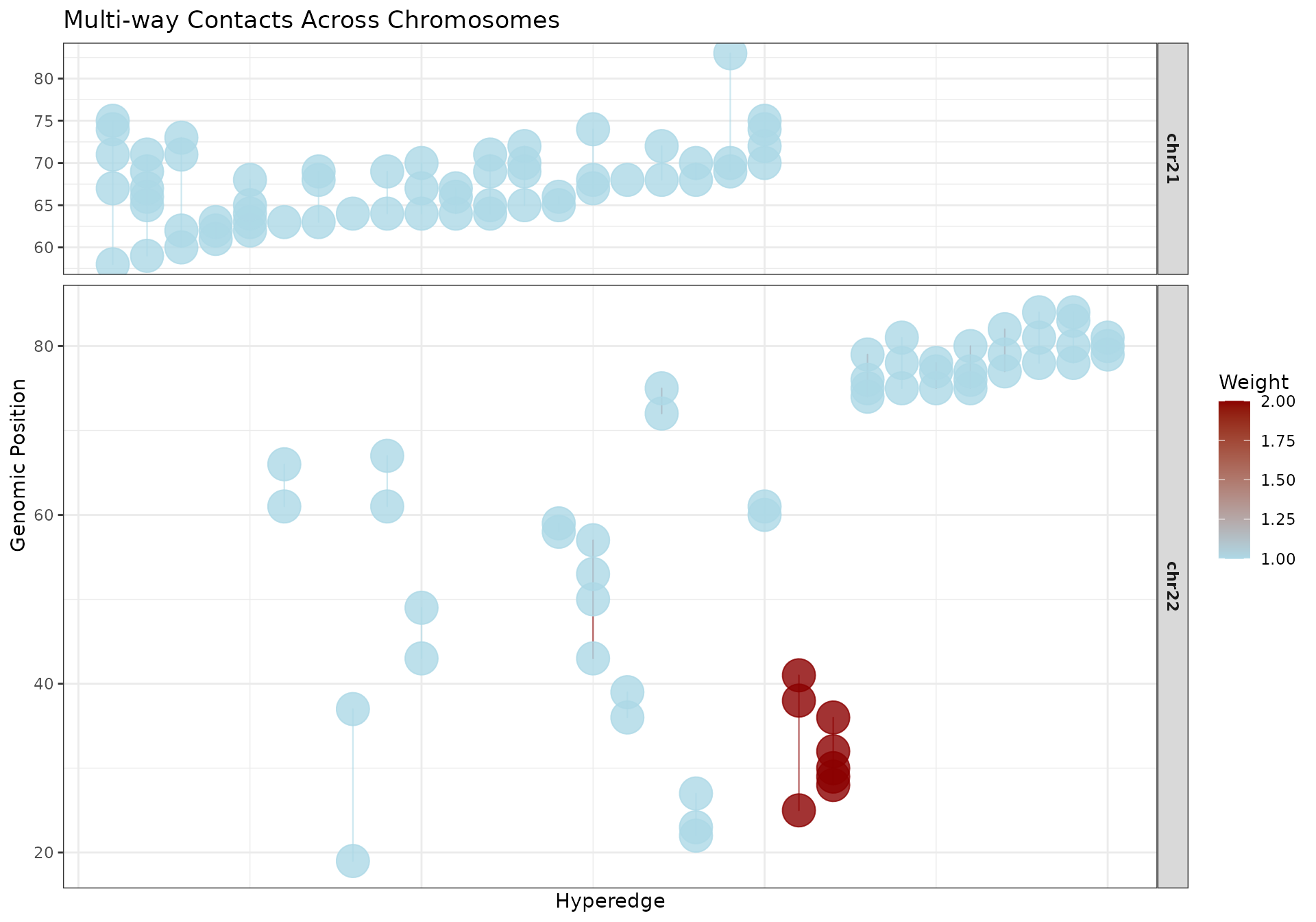
ggplot2::ggplot(
  df_multi,
  ggplot2::aes(x = x, y = bin, group = hyperedge_idx)
) +
  geom_hypergraph(
    ggplot2::aes(colour = weight),
    line_width = 0.4,
    point_size = 2
  ) +
  ggplot2::scale_color_gradient(
    low = "lightblue",
    high = "darkred",
    name = "Weight"
  ) +
  ggplot2::facet_grid(chrom ~ ., scales = "free_y", space = "free_y") +
  ggplot2::labs(
    title = "Multi-way Contacts Across Chromosomes",
    x = "Hyperedge",
    y = "Genomic Position"
  ) +
  ggplot2::theme_bw() +
  ggplot2::theme(
    strip.text = ggplot2::element_text(face = "bold"),
    axis.text.x = ggplot2::element_blank(),
    axis.ticks.x = ggplot2::element_blank()
  )

Hypergraph visualization

Adding Annotations

# Add regions of interest
regions_of_interest <- data.frame(
  ymin = c(20, 60),
  ymax = c(30, 70),
  label = c("Region A", "Region B")
)

ggplot2::ggplot(df, ggplot2::aes(x = x, y = y, group = hyperedge_idx)) +
  # Add shaded regions
  ggplot2::geom_rect(
    data = regions_of_interest,
    ggplot2::aes(xmin = -Inf, xmax = Inf, ymin = ymin, ymax = ymax),
    fill = "yellow", alpha = 0.2, inherit.aes = FALSE
  ) +
  # Add hypergraph
  geom_hypergraph(
    ggplot2::aes(colour = n_multiways),
    line_width = 0.4,
    line_alpha = 0.7
  ) +
  # Add region labels
  ggplot2::geom_text(
    data = regions_of_interest,
    ggplot2::aes(x = max(df$x) * 0.95, y = (ymin + ymax) / 2, label = label),
    hjust = 1, fontface = "bold", inherit.aes = FALSE
  ) +
  ggplot2::scale_color_viridis_c(name = "Contacts") +
  ggplot2::labs(
    title = "Hypergraph with Annotated Regions",
    x = "Hyperedge",
    y = "Genomic Bin"
  ) +
  ggplot2::theme_minimal()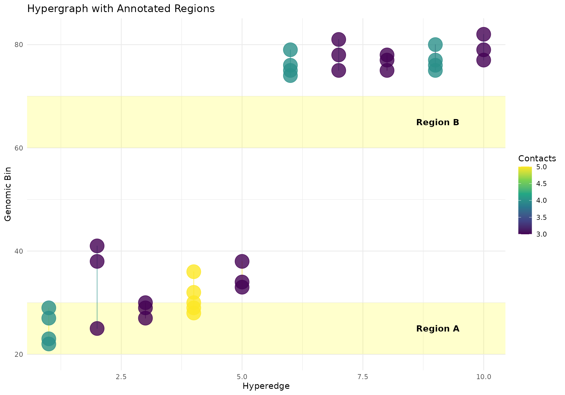

Hypergraph visualization

Highlighting Specific Hyperedges

# Highlight high-order contacts (≥5-way)
df_highlight <- df |>
  dplyr::mutate(
    is_high_order = n_multiways >= 5,
    alpha_value = ifelse(is_high_order, 0.9, 0.3),
    line_color = ifelse(is_high_order, "red", "gray70")
  )

ggplot2::ggplot(
  df_highlight,
  ggplot2::aes(x = x, y = y, group = hyperedge_idx)
) +
  geom_hypergraph(
    ggplot2::aes(colour = line_color, alpha = alpha_value),
    line_width = 0.4,
    point_size = 2
  ) +
  ggplot2::scale_color_identity() +
  ggplot2::scale_alpha_identity() +
  ggplot2::labs(
    title = "Highlighting High-Order Contacts (≥5-way)",
    subtitle = "Red = high-order, Gray = lower-order",
    x = "Hyperedge",
    y = "Genomic Bin"
  ) +
  ggplot2::theme_minimal()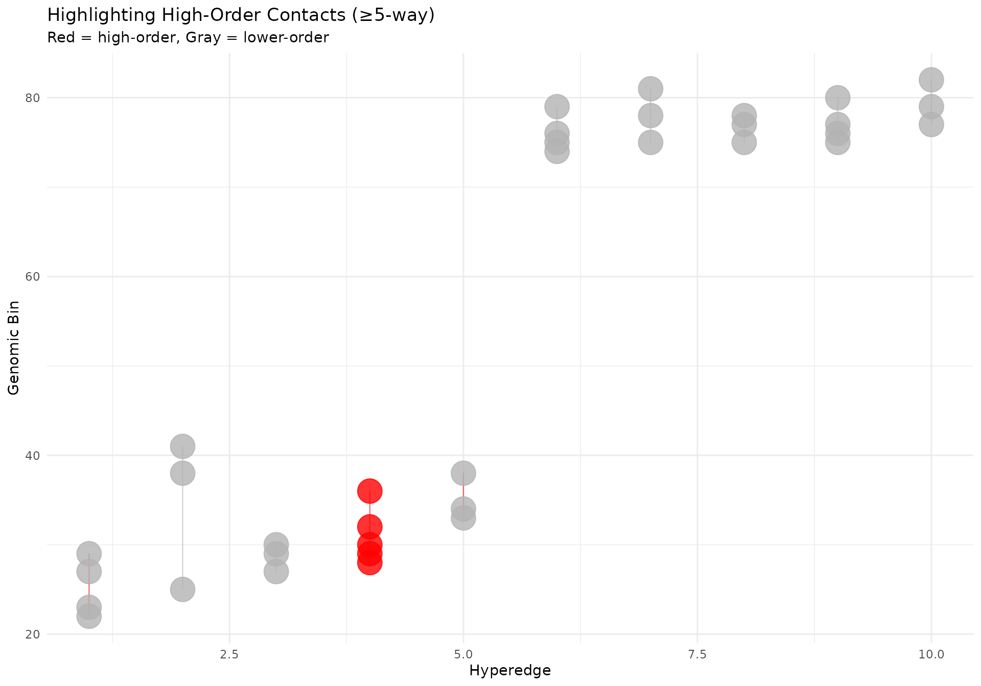

Hypergraph visualization

geom_hypergraph Parameters

The geom_hypergraph() layer accepts these key parameters:

line_width: Width of hyperedge lines (default: 0.3)
line_alpha: Transparency of lines (default: 0.6)
point_size: Size of bin points (default: 2)
point_alpha: Transparency of points (default: 0.8)
colour_by: What to color by (“n_contacts” or “none”)

You can also map aesthetics directly using aes():

colour: Color by any variable
group: Must be the hyperedge identifier
x, y: Position mappings

Cleanup

# Remove temporary file
unlink(pairs_file)

Session Info

sessionInfo()
#> R version 4.5.2 (2025-10-31)
#> Platform: x86_64-pc-linux-gnu
#> Running under: Ubuntu 24.04.3 LTS
#> 
#> Matrix products: default
#> BLAS:   /usr/lib/x86_64-linux-gnu/openblas-pthread/libblas.so.3 
#> LAPACK: /usr/lib/x86_64-linux-gnu/openblas-pthread/libopenblasp-r0.3.26.so;  LAPACK version 3.12.0
#> 
#> locale:
#>  [1] LC_CTYPE=C.UTF-8       LC_NUMERIC=C           LC_TIME=C.UTF-8       
#>  [4] LC_COLLATE=C.UTF-8     LC_MONETARY=C.UTF-8    LC_MESSAGES=C.UTF-8   
#>  [7] LC_PAPER=C.UTF-8       LC_NAME=C              LC_ADDRESS=C          
#> [10] LC_TELEPHONE=C         LC_MEASUREMENT=C.UTF-8 LC_IDENTIFICATION=C   
#> 
#> time zone: UTC
#> tzcode source: system (glibc)
#> 
#> attached base packages:
#> [1] stats     graphics  grDevices utils     datasets  methods   base     
#> 
#> other attached packages:
#> [1] gghic_0.2.1   ggplot2_4.0.1 dplyr_1.1.4  
#> 
#> loaded via a namespace (and not attached):
#>  [1] SummarizedExperiment_1.40.0 gtable_0.3.6               
#>  [3] rjson_0.2.23                xfun_0.56                  
#>  [5] bslib_0.9.0                 htmlwidgets_1.6.4          
#>  [7] rhdf5_2.54.1                Biobase_2.70.0             
#>  [9] lattice_0.22-7              bitops_1.0-9               
#> [11] rhdf5filters_1.22.0         vctrs_0.7.0                
#> [13] tools_4.5.2                 generics_0.1.4             
#> [15] parallel_4.5.2              stats4_4.5.2               
#> [17] curl_7.0.0                  tibble_3.3.1               
#> [19] pkgconfig_2.0.3             Matrix_1.7-4               
#> [21] RColorBrewer_1.1-3          cigarillo_1.0.0            
#> [23] S7_0.2.1                    desc_1.4.3                 
#> [25] S4Vectors_0.48.0            lifecycle_1.0.5            
#> [27] compiler_4.5.2              farver_2.1.2               
#> [29] Rsamtools_2.26.0            Biostrings_2.78.0          
#> [31] textshaping_1.0.4           codetools_0.2-20           
#> [33] Seqinfo_1.0.0               InteractionSet_1.38.0      
#> [35] htmltools_0.5.9             sass_0.4.10                
#> [37] RCurl_1.98-1.17             yaml_2.3.12                
#> [39] tidyr_1.3.2                 crayon_1.5.3               
#> [41] pillar_1.11.1               pkgdown_2.2.0              
#> [43] jquerylib_0.1.4             BiocParallel_1.44.0        
#> [45] cachem_1.1.0                DelayedArray_0.36.0        
#> [47] abind_1.4-8                 tidyselect_1.2.1           
#> [49] digest_0.6.39               purrr_1.2.1                
#> [51] restfulr_0.0.16             labeling_0.4.3             
#> [53] fastmap_1.2.0               grid_4.5.2                 
#> [55] cli_3.6.5                   SparseArray_1.10.8         
#> [57] magrittr_2.0.4              S4Arrays_1.10.1            
#> [59] utf8_1.2.6                  dichromat_2.0-0.1          
#> [61] XML_3.99-0.20               withr_3.0.2                
#> [63] scales_1.4.0                rmarkdown_2.30             
#> [65] XVector_0.50.0              httr_1.4.7                 
#> [67] matrixStats_1.5.0           ragg_1.5.0                 
#> [69] evaluate_1.0.5              knitr_1.51                 
#> [71] BiocIO_1.20.0               GenomicRanges_1.62.1       
#> [73] IRanges_2.44.0              viridisLite_0.4.2          
#> [75] rtracklayer_1.70.1          rlang_1.1.7                
#> [77] Rcpp_1.1.1                  glue_1.8.0                 
#> [79] BiocGenerics_0.56.0         jsonlite_2.0.0             
#> [81] R6_2.6.1                    Rhdf5lib_1.32.0            
#> [83] GenomicAlignments_1.46.0    MatrixGenerics_1.22.0      
#> [85] systemfonts_1.3.1           fs_1.6.6

Minghao Jiang

2026-01-23

Overview

Key Concepts

What is a Hypergraph?

Why Use Hypergraphs?

Filtering Strategy

Getting Started

Example Data Format

Prepare Example Data

Workflow with MultiWayContacts

Single Chromosome Analysis

Multiple Chromosomes

Method Details

import()

build()

tidy()

select()

gghypergraph()

Other Examples

Filtering by Contact Order

Comparing Chromosomes

Customizing Plots

Interpreting Results

Contact Order Distribution

Intra vs Inter-chromosomal

Best Practices

Using geom_hypergraph for Custom Plots

Basic Usage

Multi-Chromosome with Custom Layout

Adding Annotations

Highlighting Specific Hyperedges

geom_hypergraph Parameters

Cleanup

Session Info