Resolution Depth Analysis for Hi-C/-like Data

Overview

This vignette demonstrates how to analyze Hi-C pairs data to find optimal genomic resolutions using gghic’s resolution depth functions. You’ll learn how to:

Calculate contact depth at different bin sizes
Assess genome coverage across resolutions
Find optimal resolution that balances detail and completeness
Visualize tradeoffs between resolution and coverage

When to Use These Functions

These functions are essential for:

Pore-C & long-read data: Determining the best resolution for long DNA-DNA interactions
Hi-C QC: Assessing data quality and sequencing depth
Resource planning: Finding the sweet spot before expensive downstream analysis
Publication standards: Communicating data completeness to reviewers

Getting Started

Load required libraries:

load_pkg <- function(pkgs) {
  for (pkg in pkgs) suppressMessages(require(pkg, character.only = TRUE))
}

load_pkg(c("readr", "dplyr", "rappdirs", "gghic"))
#> Warning in library(package, lib.loc = lib.loc, character.only = TRUE,
#> logical.return = TRUE, : there is no package called 'readr'

Example Data

We’ll create synthetic pairs data for demonstration. In practice, load from your contact matrix file:

# Create example pairs dataset
set.seed(42)
n_interactions <- 10000

pairs <- data.frame(
  read_name = paste0("read_", seq_len(n_interactions)),
  chrom1 = sample(c("chr1", "chr2", "chr3"), n_interactions, replace = TRUE),
  pos1 = sample(1e6:10e6, n_interactions, replace = TRUE),
  chrom2 = sample(c("chr1", "chr2", "chr3"), n_interactions, replace = TRUE),
  pos2 = sample(1e6:10e6, n_interactions, replace = TRUE)
)

glimpse(pairs)
#> Rows: 10,000
#> Columns: 5
#> $ read_name <chr> "read_1", "read_2", "read_3", "read_4", "read_5", "read_6", …
#> $ chrom1    <chr> "chr1", "chr1", "chr1", "chr1", "chr2", "chr2", "chr2", "chr…
#> $ pos1      <int> 7501652, 9834771, 7511178, 9988046, 2376108, 8056778, 991689…
#> $ chrom2    <chr> "chr3", "chr1", "chr1", "chr2", "chr1", "chr2", "chr3", "chr…
#> $ pos2      <int> 4068533, 1789229, 6896113, 6916211, 7349759, 9964631, 150451…

Expected column format:

read_name: Unique identifier for each interaction
chrom1, chrom2: Chromosome names (e.g., “chr1”)
pos1, pos2: Genomic positions in base pairs
Optional: strand, mapping quality, fragment ID (ignored by analysis functions)

Choosing Your Approach

The gghic package provides two complementary approaches for analyzing pairs data:

Approach	Memory	Speed	When to Use
In-memory `calculateResolutionDepth()`	O(interactions)	Fastest	Files < 50% RAM, interactive analysis
Chunked `calcResDepthChunked()`	O(unique bins)	Fast	Files > 50% RAM, automated pipelines

In-Memory Processing (Smaller Files) - Load entire dataset into memory - Single file read (fastest) - Typical memory: ~4 bytes per interaction - Best for: Interactive exploration, visualization

Chunked Streaming (Large Files) - Read file in streaming fashion - Minimal memory footprint (~100 MB even for 100 GB files) - C-accelerated file I/O - Automatic gzip decompression - Best for: Production pipelines, server environments, very large datasets

Decision Rule: If your file size > available RAM / 2, use chunked functions.

Step 1: Calculate Resolution Depth

The calculateResolutionDepth() function bins genomic positions and counts unique interactions per bin:

# Calculate depth at 10kb resolution
depth_10kb <- calculateResolutionDepth(pairs, bin_size = 10000)

depth_10kb
#> # A tibble: 2,699 × 3
#>    chrom   bin count
#>    <chr> <int> <int>
#>  1 chr1    845    12
#>  2 chr2    812     6
#>  3 chr3    779     7
#>  4 chr1    846     7
#>  5 chr2    813     6
#>  6 chr3    780     4
#>  7 chr1    847     7
#>  8 chr3    781     8
#>  9 chr2    814     6
#> 10 chr1    848     9
#> # ℹ 2,689 more rows

# Summary statistics
summary(depth_10kb$count)
#>    Min. 1st Qu.  Median    Mean 3rd Qu.    Max. 
#>    1.00    5.00    7.00    7.41    9.00   19.00

What this returns:

chrom: Chromosome name
bin: Bin number (position / bin_size, rounded up)
count: Number of unique interactions in this bin

Interpreting the results:

High counts = well-sequenced regions
Low counts = sparse or unmappable regions
Zero-count bins = gaps (excluded from output)

Step 2: Assess Genome Coverage

The calculateGenomeCoverage() function determines what fraction of bins meet a minimum contact threshold:

# Calculate coverage at multiple resolutions
resolutions <- c(5e3, 10e3, 25e3, 50e3, 100e3, 500e3)

coverage_df <- data.frame(
  resolution_kb = resolutions / 1e3,
  n_bins = NA,
  coverage = NA
)

for (i in seq_along(resolutions)) {
  depth <- calculateResolutionDepth(pairs, resolutions[i])
  coverage_df$n_bins[i] <- nrow(depth)
  coverage_df$coverage[i] <- calculateGenomeCoverage(
    pairs, resolutions[i],
    min_contacts = 50
  )
}

coverage_df$coverage_pct <- sprintf("%.1f%%", coverage_df$coverage * 100)

coverage_df
#>   resolution_kb n_bins   coverage coverage_pct
#> 1             5   5273 0.00000000         0.0%
#> 2            10   2699 0.00000000         0.0%
#> 3            25   1080 0.00000000         0.0%
#> 4            50    540 0.02777778         2.8%
#> 5           100    270 0.99629630        99.6%
#> 6           500     54 1.00000000       100.0%

Interpreting coverage:

High coverage (>80%) at small bins: Well-sequenced, good resolution potential
Low coverage (<50%) at large bins: Sparse data, may need deeper sequencing
Coverage curve shape: Shows sequencing depth and data quality

Step 3: Find Optimal Resolution

Use binary search to find the smallest bin size achieving your target coverage:

# Find resolution with ~80% coverage
optimal_bin <- findOptimalResolution(
  pairs,
  min_bin = 1e3, # Start at 1 Kb
  max_bin = 1e6, # Search up to 1 Mb
  target_coverage = 0.8,
  min_contacts = 50
)
#> Iteration 1: Testing bin size 500,500 bp: 98.18% coverage
#> Iteration 2: Testing bin size 250,749 bp: 97.30% coverage
#> Iteration 3: Testing bin size 125,874 bp: 97.72% coverage
#> Iteration 4: Testing bin size 63,436 bp: 36.60% coverage
#> Iteration 5: Testing bin size 94,655 bp: 97.92% coverage
#> Iteration 6: Testing bin size 79,045 bp: 88.41% coverage
#> Iteration 7: Testing bin size 71,240 bp: 64.83% coverage
#> Iteration 8: Testing bin size 75,142 bp: 77.13% coverage
#> Iteration 9: Testing bin size 77,093 bp: 83.85% coverage
#> Iteration 10: Testing bin size 76,117 bp: 81.23% coverage
#> Iteration 11: Testing bin size 75,629 bp: 78.61% coverage
#> Iteration 12: Testing bin size 75,873 bp: 81.23% coverage
#> Iteration 13: Testing bin size 75,751 bp: 79.55% coverage
#> Iteration 14: Testing bin size 75,812 bp: 79.27% coverage
#> Iteration 15: Testing bin size 75,842 bp: 80.67% coverage
#> Iteration 16: Testing bin size 75,827 bp: 80.39% coverage
#> Iteration 17: Testing bin size 75,819 bp: 79.83% coverage
#> Iteration 18: Testing bin size 75,823 bp: 80.11% coverage
#> Iteration 19: Testing bin size 75,821 bp: 79.55% coverage
#> Iteration 20: Testing bin size 75,822 bp: 79.55% coverage

cat(sprintf(
  "Optimal bin size: %d bp (%.1f Kb)\n", optimal_bin, optimal_bin / 1000
))
#> Optimal bin size: 75823 bp (75.8 Kb)

# Verify the result
actual_coverage <- calculateGenomeCoverage(
  pairs, optimal_bin,
  min_contacts = 50
)
cat(sprintf("Actual coverage: %.2f%%\n", actual_coverage * 100))
#> Actual coverage: 80.11%

How it works:

Binary search across the bin size range
Tests each candidate bin size
Returns smallest bin that meets target coverage
Typically completes in 10-15 iterations

Pro tip: Start with target_coverage = 0.8 (80%). Adjust based on your analysis needs.

Step 4: Visualize Coverage Distribution

Create a boxplot showing how contact counts vary across resolutions:

plotResolutionCoverage(
  pairs,
  bin_sizes = c(5e3, 10e3, 25e3, 50e3, 100e3, 500e3),
  min_contacts = 50,
  title = "Contact Distribution by Resolution"
)

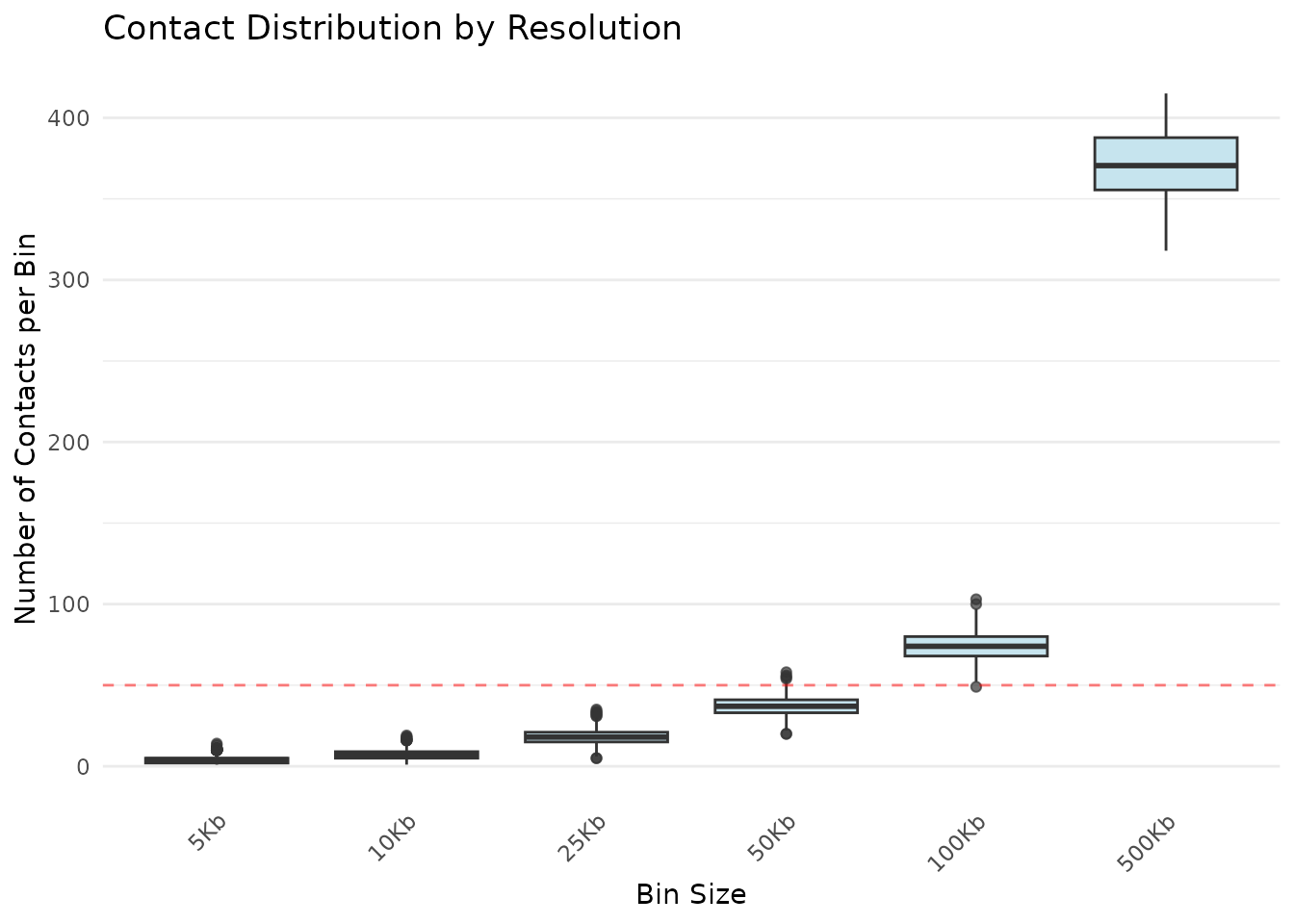
Distribution of contacts per bin at different resolutions

What to look for:

Widening boxes: Decreasing contacts with larger bins (expected)
Outliers (dots): Unusually enriched regions (e.g., centromeres, pericentromeres)
Median position: Typical coverage at that resolution
Whisker length: Range of contact values (high whiskers = variable coverage)

Step 5: Plot Coverage vs Resolution

Create a line plot showing how coverage changes with resolution:

plotCoverageCurve(
  pairs,
  bin_sizes = c(5e3, 10e3, 25e3, 50e3, 100e3, 500e3, 1e6),
  min_contacts = 50,
  title = "Coverage vs Resolution"
)

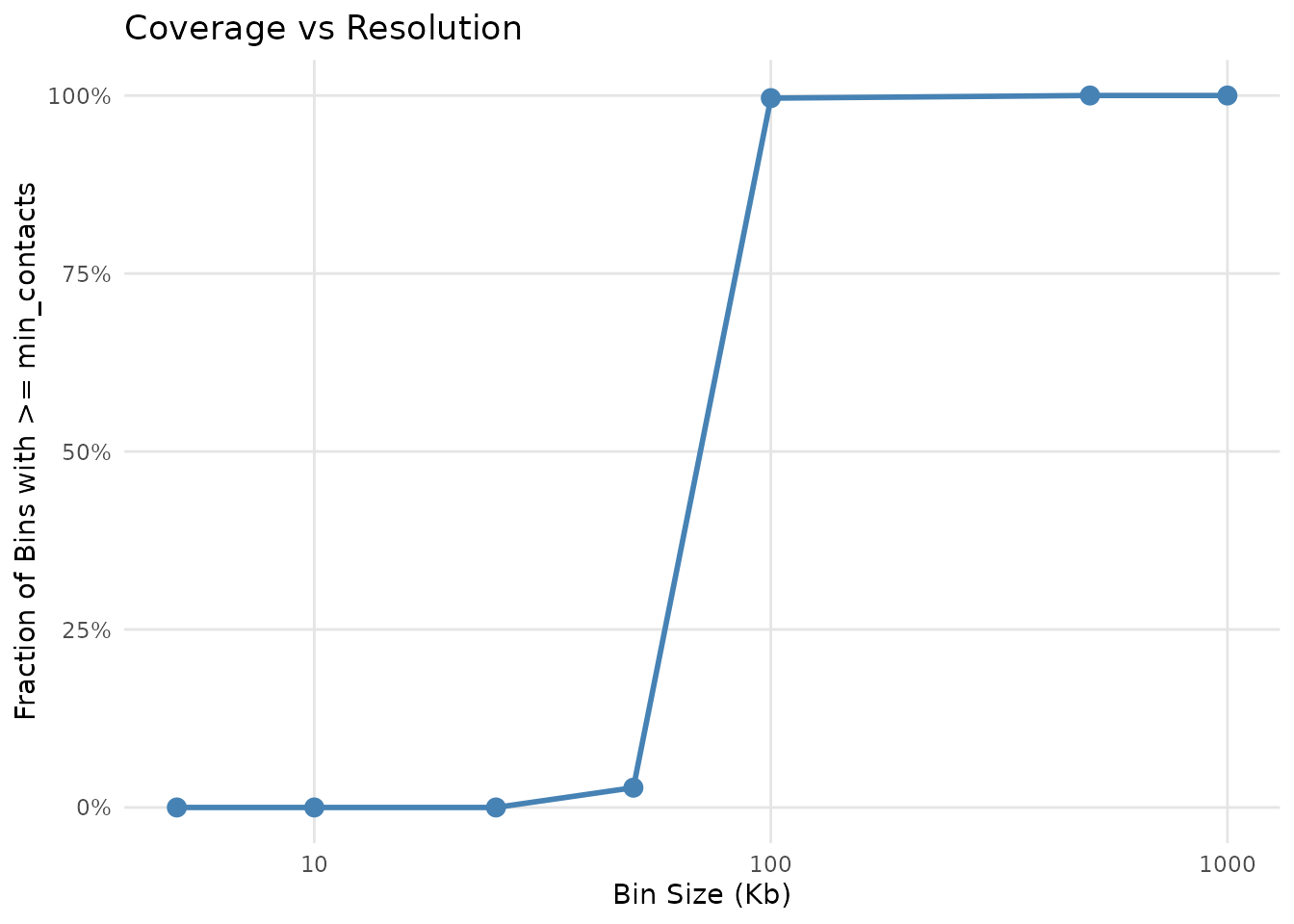
Genome coverage as a function of bin size

Curve interpretation:

Sharp drop at small bins: Limited sequencing depth
Plateau region: Where additional bin size doesn’t improve coverage much
“Knee” of curve: The optimal resolution sweet spot
Steep regions: Good resolution potential at that bin size

Processing Large Files (100 GB+)

⚠️ Note: The code examples in this section are provided for reference but are not executed in this vignette.

For files that don’t fit in R memory, use the _chunked variants which stream the file with C-level I/O:

# Download example file with caching
cache_dir <- rappdirs::user_cache_dir("gghic")
dir.create(cache_dir, recursive = TRUE, showWarnings = FALSE)

pairs_file <- file.path(cache_dir, "test.txt.gz")
download_url <- "https://www.dropbox.com/scl/fi/yc4axg1mf2i9zylg3d0oe/test.txt.gz?rlkey=sdsdhsnixo01koo38d242y4c8&st=t4rn0js0&dl=1"

if (!file.exists(pairs_file)) {
  message("Downloading test data to cache directory...")
  download.file(
    download_url, pairs_file,
    method = "auto", quiet = TRUE
  )
  message("Downloaded to: ", pairs_file)
} else {
  message("Using cached file: ", pairs_file)
}

Approach 1: Direct File Reading (Simple but Slower)

Read the file each time a function is called:

# Each function reads the file independently
opt_bin <- findOptResChunked(
  pairs_file = pairs_file,
  min_bin = 1e3,
  max_bin = 5e4,
  target_coverage = 0.8,
  min_contacts = 1000
)

# Reads file again
coverage <- calcGenomeCovChunked(
  pairs_file = pairs_file,
  bin_size = opt_bin,
  min_contacts = 1000
)

# Reads file again
depth <- calcResDepthChunked(
  pairs_file = pairs_file,
  bin_size = opt_bin
)

Problem: For a 10 GB file, you’re reading 10 GB three times (30 GB total I/O)!

Approach 2: Cache Once, Reuse Many Times (FASTEST!)

Read the file once into C memory, then reuse the cached data:

# 1. READ FILE INTO C MEMORY ONCE ----
# This takes time initially but creates a persistent cache
cache <- readPairsCache(pairs_file)
cat("File loaded into C memory cache\n")

# 2. FIND OPTIMAL RESOLUTION (using cache) ----
# This is now instant - no file I/O!
opt_bin <- findOptResChunked(
  cache = cache,
  min_bin = 1e3,
  max_bin = 5e4,
  target_coverage = 0.8,
  min_contacts = 1000
)
cat("Optimal resolution:", opt_bin / 1e3, "Kb\n")

# 3. CHECK COVERAGE (using cache) ----
# Also instant!
coverage <- calcGenomeCovChunked(
  cache = cache,
  bin_size = opt_bin,
  min_contacts = 1000
)
cat("Coverage:", sprintf("%.1f%%\n", coverage * 100))

# 4. EXTRACT BINNED DEPTHS (using cache) ----
# Still instant!
depth <- calcResDepthChunked(
  cache = cache,
  bin_size = opt_bin
)

# 5. TRY DIFFERENT BIN SIZES (no additional I/O!) ----
depth_5kb <- calcResDepthChunked(cache = cache, bin_size = 5000)
depth_10kb <- calcResDepthChunked(cache = cache, bin_size = 10000)
depth_50kb <- calcResDepthChunked(cache = cache, bin_size = 50000)

# Cache is automatically freed when removed or R session ends
rm(cache)
gc()

Performance: For a 10 GB file: - Without cache: ~30 seconds × 3 operations = 90 seconds - With cache: ~30 seconds (once) + ~0.1 seconds × operations = 30 seconds

3x faster! And the speedup increases with more operations.

Approach 3: Get Cache from findOptResChunked

Let findOptResChunked() return the cache for subsequent use:

# Find optimal resolution and get cache back
result <- findOptResChunked(
  pairs_file = pairs_file,
  min_bin = 1e3,
  max_bin = 5e4,
  target_coverage = 0.8,
  min_contacts = 1000,
  return_cache = TRUE # Get the cache back!
)

# Extract results
opt_bin <- result$bin_size
cache <- result$cache

cat("Optimal resolution:", opt_bin / 1e3, "Kb\n")

# Now reuse the cache for other operations
coverage <- calcGenomeCovChunked(
  cache = cache,
  bin_size = opt_bin,
  min_contacts = 1000
)

depth <- calcResDepthChunked(
  cache = cache,
  bin_size = opt_bin
)

When to Use Each Approach

Approach	Best For	I/O Operations
Direct File	Single analysis, simple scripts	N operations
Explicit Cache	Interactive exploration, multiple analyses	1 operation
Return Cache	When starting with `findOptResChunked()`	1 operation

Rule of thumb: If you’ll call more than one chunked function, use the cache!

Interpreting Your Results

What the Coverage Curve Tells You

Sharp drop at small bins - Data is sparse at high resolution - Limited sequencing depth or short reads - Consider deeper sequencing or larger bins

Plateau region - Coverage maxes out (can’t improve by increasing bin size) - Indicates natural sequencing depth ceiling - Optimal resolution likely at transition point

High coverage at large bins (>80%) - Well-sequenced dataset - Can use smaller bins safely - Good candidate for publication-quality analysis

Low coverage at large bins (<50%) - Sparse data - May need additional sequencing - Consider quality filtering

Choosing Target Coverage

Exploration: 50-60% (quick, uses fewer bins)
Standard analysis: 75-85% (good balance)
Publication: 85-90%+ (most stringent)

Higher coverage = higher confidence but requires more sequencing.

Next Steps

Once you’ve found your optimal resolution, explore other gghic functions for visualization:

geom_hic(): Create interaction scatter plots
geom_loop(): Highlight chromatin loops
geom_tad(): Show topologically associating domains
geom_ideogram(): Add chromosome context
theme_hic(): Specialized theme for Hi-C plots

See the main gghic vignette for complete examples.

FAQ

Q: Why does coverage decrease with larger bins? A: By definition—larger bins aggregate more positions but contact counts don’t increase proportionally. Coverage measures the fraction of bins with sufficient contacts.

Q: Should I use chunked functions for small files? A: No, use in-memory functions—they’re simpler and faster for files that fit in RAM.

Q: Can I use these functions on non-Hi-C data? A: Yes, any “pairs” data with (chrom, position) coordinates works: Pore-C, 4C, 5C, etc.

Session Info

sessionInfo()
#> R version 4.5.2 (2025-10-31)
#> Platform: x86_64-pc-linux-gnu
#> Running under: Ubuntu 24.04.3 LTS
#> 
#> Matrix products: default
#> BLAS:   /usr/lib/x86_64-linux-gnu/openblas-pthread/libblas.so.3 
#> LAPACK: /usr/lib/x86_64-linux-gnu/openblas-pthread/libopenblasp-r0.3.26.so;  LAPACK version 3.12.0
#> 
#> locale:
#>  [1] LC_CTYPE=C.UTF-8       LC_NUMERIC=C           LC_TIME=C.UTF-8       
#>  [4] LC_COLLATE=C.UTF-8     LC_MONETARY=C.UTF-8    LC_MESSAGES=C.UTF-8   
#>  [7] LC_PAPER=C.UTF-8       LC_NAME=C              LC_ADDRESS=C          
#> [10] LC_TELEPHONE=C         LC_MEASUREMENT=C.UTF-8 LC_IDENTIFICATION=C   
#> 
#> time zone: UTC
#> tzcode source: system (glibc)
#> 
#> attached base packages:
#> [1] stats     graphics  grDevices utils     datasets  methods   base     
#> 
#> other attached packages:
#> [1] gghic_0.2.1    rappdirs_0.3.4 dplyr_1.1.4   
#> 
#> loaded via a namespace (and not attached):
#>  [1] SummarizedExperiment_1.40.0 gtable_0.3.6               
#>  [3] rjson_0.2.23                xfun_0.56                  
#>  [5] bslib_0.9.0                 ggplot2_4.0.1              
#>  [7] htmlwidgets_1.6.4           rhdf5_2.54.1               
#>  [9] Biobase_2.70.0              lattice_0.22-7             
#> [11] bitops_1.0-9                rhdf5filters_1.22.0        
#> [13] vctrs_0.7.0                 tools_4.5.2                
#> [15] generics_0.1.4              parallel_4.5.2             
#> [17] stats4_4.5.2                curl_7.0.0                 
#> [19] tibble_3.3.1                pkgconfig_2.0.3            
#> [21] Matrix_1.7-4                RColorBrewer_1.1-3         
#> [23] cigarillo_1.0.0             S7_0.2.1                   
#> [25] desc_1.4.3                  S4Vectors_0.48.0           
#> [27] lifecycle_1.0.5             compiler_4.5.2             
#> [29] farver_2.1.2                Rsamtools_2.26.0           
#> [31] Biostrings_2.78.0           textshaping_1.0.4          
#> [33] codetools_0.2-20            Seqinfo_1.0.0              
#> [35] InteractionSet_1.38.0       htmltools_0.5.9            
#> [37] sass_0.4.10                 RCurl_1.98-1.17            
#> [39] yaml_2.3.12                 tidyr_1.3.2                
#> [41] crayon_1.5.3                pillar_1.11.1              
#> [43] pkgdown_2.2.0               jquerylib_0.1.4            
#> [45] BiocParallel_1.44.0         DelayedArray_0.36.0        
#> [47] cachem_1.1.0                abind_1.4-8                
#> [49] tidyselect_1.2.1            digest_0.6.39              
#> [51] purrr_1.2.1                 restfulr_0.0.16            
#> [53] labeling_0.4.3              fastmap_1.2.0              
#> [55] grid_4.5.2                  cli_3.6.5                  
#> [57] SparseArray_1.10.8          magrittr_2.0.4             
#> [59] S4Arrays_1.10.1             utf8_1.2.6                 
#> [61] dichromat_2.0-0.1           XML_3.99-0.20              
#> [63] withr_3.0.2                 scales_1.4.0               
#> [65] rmarkdown_2.30              XVector_0.50.0             
#> [67] httr_1.4.7                  matrixStats_1.5.0          
#> [69] ragg_1.5.0                  evaluate_1.0.5             
#> [71] knitr_1.51                  BiocIO_1.20.0              
#> [73] GenomicRanges_1.62.1        IRanges_2.44.0             
#> [75] rtracklayer_1.70.1          rlang_1.1.7                
#> [77] Rcpp_1.1.1                  glue_1.8.0                 
#> [79] BiocGenerics_0.56.0         jsonlite_2.0.0             
#> [81] R6_2.6.1                    Rhdf5lib_1.32.0            
#> [83] GenomicAlignments_1.46.0    MatrixGenerics_1.22.0      
#> [85] systemfonts_1.3.1           fs_1.6.6

Minghao Jiang

2026-01-23